Abaqus Heat Transfer Tutorial Step By Step

In Abaqus, heat transfer problems are solved using the energy balance equation and constitutive laws for heat conduction, convection, and radiation. Below are the key equations, assumptions, and boundary conditions typically used for thermal analysis in Abaqus.

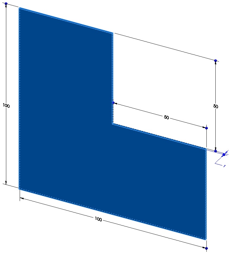
Problem definition:

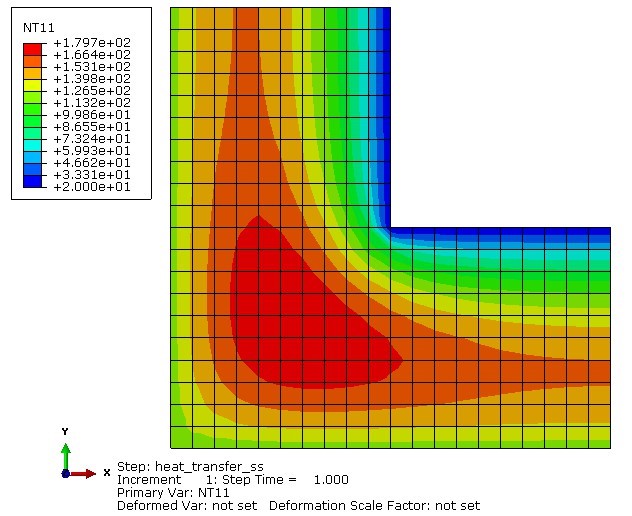
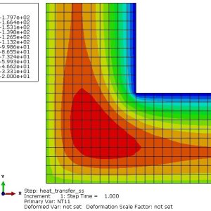
The thin “L‐shaped” steel part shown above (lengths in meters) is exposed to a temperature of 20 centigrade degrees on the two surfaces of the inner corner, and 120 centigrade degrees on the two surfaces of the outer corner. A heat flux of 10 W/m2 is applied to the top surface. Treat the remaining surfaces as insulated.

Heat Transfer Governing Equations in Abaqus

The general heat transfer equation solved by Abaqus is derived from the energy conservation principle:

ρcp∂T∂t=∇⋅(k∇T)+Q+qgen

Where:

• ρ: Material density
  [mass/length3]
• cp

​: Specific heat capacity

[energy/(mass⋅temperature)]

T: Temperature [K or ∘C]

• t

: Time [s]

• k

: Thermal conductivity

[power/(length⋅temperature)]

Q : Heat flux due to convection/radiation[power/length2]

• qgen

​: Internal heat generation

[power/length3] [power/length3] (e.g., Joule heating, chemical reactions).

2. Key Assumptions

Abaqus thermal analysis relies on the following assumptions:

1. Fourier’s Law of Heat Conduction: Heat flux q

is proportional to the temperature gradient:

q=−k∇TNewton’s Law of Cooling (for convection):

qconv=h(T−Tenv)

1. • h

: Convective heat transfer coefficient

[power/(length2⋅temperature)]

[power/(length2⋅temperature)]

1. • Tenv

​: Ambient/sink temperature.

1. Stefan-Boltzmann Law (for radiation):
   qrad=ϵσ(T4−Tenv4)
   • ϵ

: Emissivity

1. • σ

: Stefan-Boltzmann constant (

5.67×10−8 W/m2K4

5.67×10−8W/m2K4 in SI).

1. Material Properties:
   • k ,ρ ,cp ,h and ϵ

ϵ are assumed constant or temperature-dependent.

1. Transient vs. Steady-State:
   •  For transient analysis:
     ∂T/∂t≠0
   • For steady-state analysis:
     ∂T/∂t=0

Heat Transfer Boundary Conditions in Abaqus

Boundary conditions are critical for solving problems:

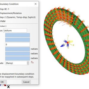
1. Dirichlet (Essential BC):
   • Prescribed temperature at surfaces:
     T=T0
2. Neumann (Natural BC):
   • Prescribed heat flux:
     q=q0
3. Convection:
   • Heat loss/gain to surroundings:
     q=h(T−Tenv)
4. Radiation:
   • Heat exchange via radiation:
     q=ϵσ(T4−Tenv4)
5. Symmetry/Axisymmetry:
   • Zero heat flux across symmetric boundaries:
     ∇T⋅n=0

4. Material Properties

Define these properties in the Abaqus material module:

• Thermal Conductivity (k )
• Density (ρ )
• Specific Heat (cp )
• Convective Coefficient (h )

(for surface interactions)

• Emissivity (ϵ )(for radiation)

5. Common Analysis Types

1. Steady-State Heat Transfer:
   • Solve
     ∇⋅(k∇T)+Q+qgen=0
   • Used for equilibrium temperature distributions.
2. Transient Heat Transfer:
   • Solve
     ρcp∂T∂t=∇⋅(k∇T)+Q+qgen
   • Requires time increments and initial conditions (
     T(t=0)
3. Coupled Thermal-Stress Analysis:
   • Solve heat transfer and mechanical deformation simultaneously (e.g., thermal expansion).

6. Key Assumptions in Abaqus

• Linear vs. Nonlinear:
  • Linear: Constant material properties (e.g.,k,
    cp
  • Nonlinear: Temperature-dependent properties.
• Radiation: Often simplified using view factors or ignored if convection dominates.
• Lumped Capacitance: Not directly used (Abaqus solves spatially varying temperature fields).