Step by Step Analysis of a Composite Sheet in Abaqus

A composite is a material composed of two or more different materials. These materials are being considered for a variety of reasons, including the low cost in the manufacturing and forming processes, low weight, higher strength-to-weight ratio, high corrosion resistance, low heat transfer coefficient, low thermal expansion coefficient, etc.
Composites are classified into several types, such as Woven, Unidirectional, Randomly Oriented Fibers, and Discrete Particles.

In Abaqus software, there are several ways to simulate composite materials. You can simulate composite materials using one of the three elements Solid, Continuum Shell, or Shell. Remember that unidirectional fiber composites are typically assumed to be orthotropic. Do you remember what orthotropic materials are and how many parameters are required to fully determine their elastic mechanical properties?

Here’s a detailed explanation of the simulation process outlined in the article, focusing on the analysis of a composite sheet in Abaqus:

1. Problem Setup and Geometry Creation

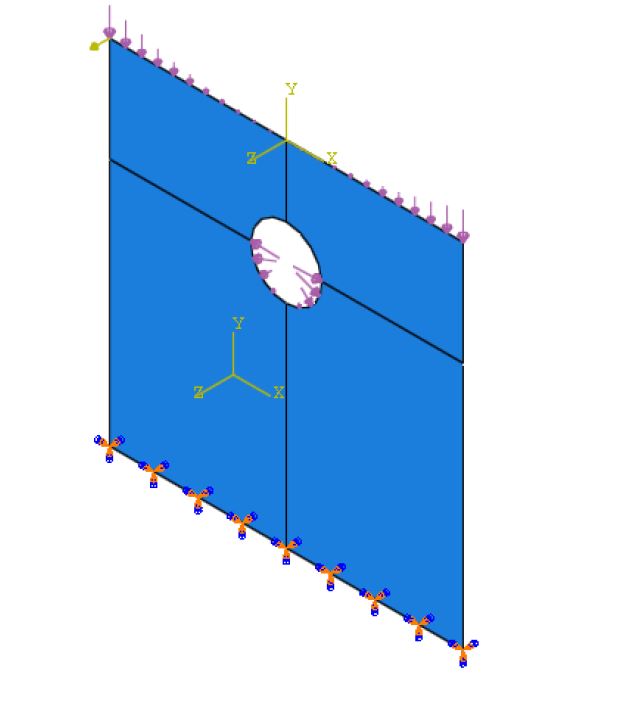
Consider a Glass-Epoxy [0,45, -45,90,0,90, -45,45, 0] composite sheet with a middle layer of Core or a light filler core, as shown in the figure 1.

Objective: Model a glass-epoxy composite sheet with a central hole and a core filler layer.

• Part Module:
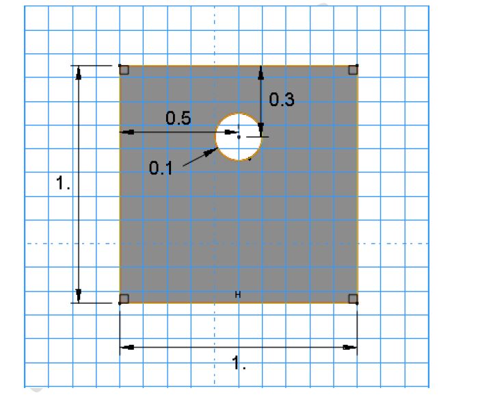
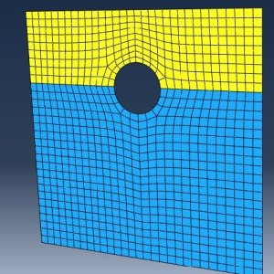
  • Create a 3D deformable shell with dimensions 1 m × 1 m.
  • Add a circular hole (diameter 0.1 m) using the Sketcher tool.
  • Partition the sheet into quadrants to facilitate structured meshing and load application.

Why?
Partitioning helps define a structured mesh and simplifies assigning local coordinate systems for non-uniform loads.

2. Material and Composite Layup Definition

Property Module:

• Material 1 (Glass-Epoxy):
  • Density: 1800 kg/m³.
  • Orthotropic elastic properties (e.g., E1,E2,G12,ν12E1​,E2​,G12​,ν12​).
• Material 2 (Core Filler):
  • Density: 800 kg/m³.
  • Isotropic properties ($E=5\text{GPa},\nu =0.3$).
• Composite Layup:
  • Define the stacking sequence: $[0,45,-45,90,0,90,-45,45,0]$.
  • Assign each layer’s thickness (1 mm for glass-epoxy, 10 mm for core) and fiber orientation.

Key Tool:
Use the Composite Layup tool to assign materials and angles to individual plies (Figure 2-3 in the article).

3. Loads and Boundary Conditions in Abaqus

Load Module:

1. Boundary Conditions:
   • Fully fix the bottom edge (Encastre constraint).
2. Applied Loads:
   • Distributed Loads:
     • Upper/lower edges: 300, ⁣000X2 N/m2300,000X2N/m2 (defined via Analytical Field).
     • Hole edge: 107X2 N/m2107X2N/m2.
   • Concentrated Force: 100 N at the left corner.
3. Coordinate System:
   • Create a local coordinate system (HOLE-CSYS) at the hole’s center to align the load equations.

Why Analytical Fields?
Analytical fields allow spatially varying loads (e.g., X2X2 dependence) to mimic real-world non-uniform loading.

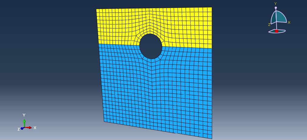
4. Meshing

Mesh Module:

• Element Type: Use S8R (8-node quadratic shell elements with reduced integration).
• Structured Mesh:
  • Seed edges around the hole with 5 divisions for refinement.
  • Mesh the entire sheet with structured quad elements.

Why Structured Meshing?
Structured meshes improve accuracy near stress-concentration zones (e.g., hole edges).

5. Job Submission and Solving

Job Module:

• Create a job named COMPOSITE-STATIC.
• Submit the job and monitor convergence using the Job Monitor.

Analysis Type:

• Static, General (for linear/nonlinear static analysis).

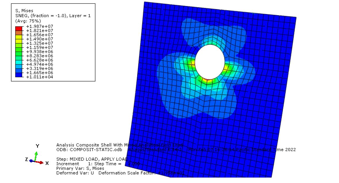
6. Post-Processing and Results

Visualization Module:

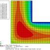
1. Stress/Strain Contours:
   • Plot von Mises stress to identify high-stress regions (Figure 8-1).
   • Visualize displacement and strain fields.
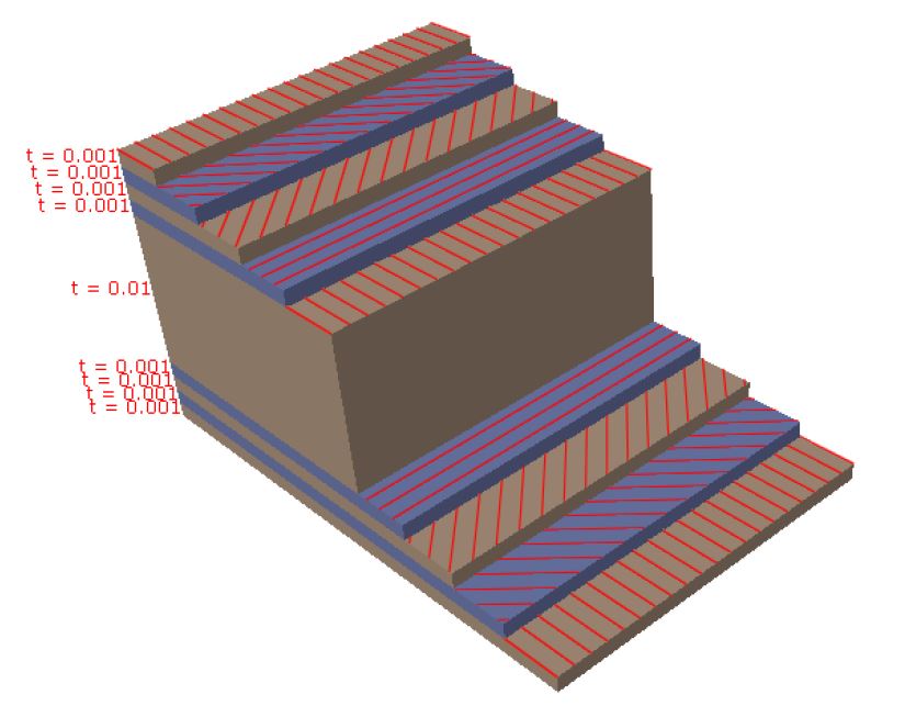
2. Ply Stack Plot:
   • Use Query → Ply Stack Plot to visualize layer orientations and thicknesses (Figure 8-2).
3. Thickness-Dependent Results:
   • Extract strain/stress through the thickness using XY Data (Figure 8-4).

Key Techniques Used

1. Non-Uniform Load Application:
   • Analytical fields with X2X2 dependence model realistic load distributions (e.g., earthquake-like loads).
2. Composite Layup Definition:
   • Assigning orthotropic properties to individual plies ensures accurate representation of fiber-dominated behavior.
3. Local Coordinate Systems:
   • Critical for aligning loads with the geometry (e.g., hole-centric loads).

Advanced Exercise: Buckling Analysis

The article includes a supplementary exercise for buckling analysis of a 16-layer composite panel under axial compression. Key steps:

1. Layup: Define the stacking sequence $\{\pm 45/90/0/0/90/45\}$.
2. Boundary Conditions: Apply uniform axial displacement ($\delta =0.803\text{mm}$).
3. Eigenvalue Analysis: Solve for buckling modes using Abaqus’ Linear Perturbation step.

Why This Workflow Matters

• Accuracy: Structured meshing and orthotropic material definitions capture composite-specific behavior.
• Realism: Non-uniform loads and layered modeling reflect industrial applications (e.g., aerospace components).
• Post-Processing: Tools like ply stack plots and XY data enable detailed failure analysis.

For further learning, the article recommends advanced tutorials on composite damage and buckling from Mathech.

This process equips engineers to simulate composites in Abaqus efficiently, from simple static analyses to complex buckling/damage scenarios.