Nonlinear Shell Analysis in Abaqus: Complete 2025 Step-by-Step Tutorial

Mastering nonlinear shell analysis in Abaqus is essential for accurately simulating real-world engineering behaviors such as buckling, large deformations, and complex material response. This complete 2025 step-by-step tutorial provides the practical, hands-on guidance you need to confidently master this advanced simulation.

In this comprehensive guide, we’ll walk you through a detailed example: modeling a curved aluminum shell under compression. You’ll learn how to simulate its nonlinear geometric response with fixed boundary conditions from start to finish.

Follow our structured approach to get accurate results from a blank page. We start with the initial setup of Abaqus nonlinear shell analysis and guide you through creating shell models, defining material properties, and configuring the nonlinear step. Then, you’ll learn how to apply boundary conditions and loads, implement effective meshing strategies, and finally, post-process the results for interpreting buckling and stresses.

By following this tutorial, you will gain a repeatable workflow to confidently complete your complex shell analysis projects.

1. Abaqus Nonlinear Shell Analysis Setup

Start your nonlinear shell simulation in Abaqus/CAE by creating a new model database. Define accurate model dimensions and save your project file to maintain a clear workflow. A well-structured setup ensures reliable and repeatable finite element analysis results.

Material Definition

Assign material properties that match your structural model:

• Young’s Modulus: 70 GPa (or 70,000 MPa in Abaqus units).
• Poisson’s Ratio: 0.3.

These values represent typical aluminum alloy behavior, suitable for nonlinear shell analysis and buckling studies in Abaqus.

Boundary Conditions

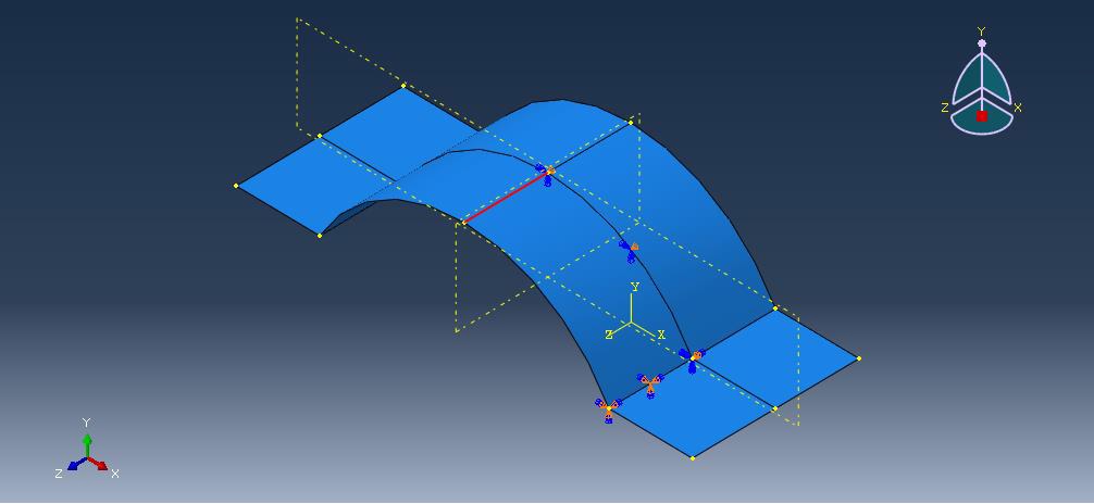
Apply boundary constraints on the horizontal edges using the Encastre condition to fully restrict all degrees of freedom. Proper boundary setup prevents unrealistic displacements and keeps the model stable during loading.

Loading Configuration

Apply a 100 MPa compressive pressure to the curved shell section. This load simulates structural stress under compression, a critical condition for nonlinear response evaluation.

By following these steps, your Abaqus model will be ready for nonlinear shell deformation analysis, providing valuable insights into structural stability and material behavior.

2. Creating Shell Models in Abaqus

Building an accurate shell geometry is the foundation of every Abaqus simulation. In this guide, you’ll learn how to create a curved shell structure using the Part module in Abaqus/CAE. Precision in geometry definition ensures reliable stress and deformation results during finite element analysis.

1. Create a New Part

• Go to Part → Create Part in the Abaqus interface.
• Set these parameters:
  • Name: Part-1
  • Modeling Space: 3D
  • Type: Deformable
  • Base Feature: Shell (Planar)
  • Approximate Size: 100 mm

These settings establish a clean, scalable model for nonlinear shell simulation.

2. Sketch the Geometry

Use the Circle tool to draw a circular base:

• Center at (0, 0)
• Radius = 10 mm

Then use the Line tool to draw lines from (15, 5) to (15, 5). Trim excess geometry to form the curved shell profile.
Add 5 mm dimensions to all key edges to maintain consistency across the model.

3. Extrude the Shell

Extrude the shell to create a 3D feature:

• Method: Blind
• Depth: 10 mm

This operation defines the shell thickness and final 3D geometry.

With this geometry complete, your model is ready for Abaqus boundary conditions and nonlinear load application. Accurate sketching minimizes meshing issues and ensures your finite element analysis produces realistic results.

3. Defining Shell Material Properties in Abaqus

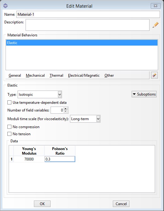
Accurate material definition is crucial for nonlinear shell analysis in Abaqus/CAE. In this step, you’ll assign aluminum properties that capture elastic and plastic behavior. Correct inputs ensure realistic stress, strain, and deformation results during finite element simulation.

1. Create the Material

• Go to Property → Create Material.
• Name: Material-1
• Under Elastic, set:
  • Young’s Modulus: 70,000 MPa
  • Poisson’s Ratio: 0.3

These parameters define the linear elastic response of aluminum alloys typically used in thin shell structures.

2. Create the Shell Section

• Go to Section → Create.
• Set Category: Shell
• Type: Homogeneous
• Shell Thickness: 1 mm
• Assign Material-1 to this section.

This defines a uniform material layer ideal for curved or thin-walled components.

3. Assign the Section to the Part

• Select your part in the model tree.
• Choose Assign Section → Section-1.

This links your material and section to the geometry, finalizing the setup for structural analysis.

A properly defined material guarantees accurate results when analyzing large-strain and nonlinear deformation. Your Abaqus model is now ready for loading and boundary condition setup.

4. Assembly Module for Shell Structures

Position your shell instance within the global coordinate system of the assembly. This step ensures all subsequent definitions like loads and BCs are applied correctly in space.

Create Instance:

1. Go to Instance → Create.
2. Select Part-1 → Independent (Mesh on Instance).

Partition Geometry:

1. Use Datum Planes to split the shell for symmetry.
2. Apply Partition Face using the created datum planes.

5. Nonlinear Step Configuration in Abaqus

Create a Static, General step and activate NLGEOM for large displacements. We configure the incrementation controls to ensure solver convergence during the nonlinear response.

Step Module:

1. Create Step:
   • Go to Step → Create.
   • Name: Step-1.
   • Type: Static, General.
   • Enable Nlgeom (Nonlinear Geometry) for large deformations.

6. Boundary Conditions for Shell Analysis

Apply realistic constraints to represent clamped edges on your shell. This section shows you how to fully restrain the necessary degrees of freedom.

Load Module:

1. Clamp Horizontal Edges:
   • Create Boundary Condition → Encastre on horizontal edges.
2. Apply Symmetry:
   • For the curved edges, apply ZSYMM (symmetry about XY-plane).
   • For mid-edges, apply XSYMM (symmetry about YZ-plane).

7. Applying Loads to Shell Structures

Define a compressive pressure load on the shell surface. You will learn how to specify the load magnitude and direction to induce buckling.

1. Pressure Load:
   • Go to Load → Create.
   • Type: Pressure.
   • Magnitude: 100 MPa.
   • Select the curved face for load application.

8. Meshing Strategies for Shell Elements

Generate a high-quality finite element mesh using S4R shell elements. We discuss global seed sizing and mesh controls to ensure accuracy without excessive computation time.

Mesh Module:

1. Seed Edges:
   • Use Seed Edges → Assign 10 elements to long edges, 5 elements to short edges.
2. Assign Element Type:
   • Select S4R (4-node shell element with reduced integration).
3. Mesh the Part:
   • Click Mesh Part Instance.

9. Running Abaqus Nonlinear Analysis Jobs

Submit your analysis job to the solver and monitor its progress for errors or warnings. A successfully completed job is the gateway to your results.

Job Module:

1. Create Job:
   • Go to Job → Create.
   • Name: Job-1.
   • Submit the job.
2. Monitor Solution:
   • Use Job Manager → Monitor to track progress.

10. Post-Processing Shell Analysis Results

Visualize the deformed shape, stress contours, and buckling mode in the Visualization module. Learn to create informative animations and plots for your engineering reports.

Visualization Module:

1. Plot Deformed Shape:
   • Click Plot Contours on Deformed Shape to visualize displacements.
2. View Stress/Strain:
   • Under Field Output, select S, Mises for von Mises stress.
   • Use Probe Values to check stress at specific elements.
3. Compare Deformed/Undeformed:
   • Enable Plot Undeformed Shape to overlay results.

11.Nonlinear Shell Analysis Best Practices

This section summarizes crucial tips for troubleshooting convergence issues and validating your results. Apply these best practices to enhance the reliability of all your future simulations.

• Units: Ensure all inputs use mm (length), MPa (stress), and N (force).
• Symmetry: Exploit symmetry to reduce model size and computation time.
• Nonlinearity: Enable Nlgeom to account for large deformations.

By following these steps, you can simulate the nonlinear behavior of a curved shell under compressive load in Abaqus. For complex models, refine the mesh or adjust solver settings for convergence.