
IS YOUR Abaqus simulation stopping before it finishes? You’re likely facing a convergence problem – one of the most common challenges in finite element analysis (FEA). A convergence problem occurs when the Abaqus solver cannot find a stable solution, causing the analysis to stop unexpectedly. These interruptions can be frustrating, especially when they happen repeatedly, wasting both time and effort.
Understanding convergence in Abaqus is essential for running reliable simulations. A converged model means the internal forces are in balance with the applied loads, allowing the analysis to proceed smoothly. When this balance breaks down, the solver cannot continue, and the simulation stops.
📘 GUIDE This guide explains why convergence fails and how you can fix it to achieve stable and accurate results.
In this guide, we’ll walk you through the main causes of convergence failure in Abaqus. The most common issues include:
For each of these issues, we provide clear and practical solutions. You’ll also find best practices to help you prevent convergence issues before they occur.
🚀 FOLLOW Follow our expert guidance to get your Abaqus simulations running smoothly again. With the right approach, you can eliminate convergence problems and achieve accurate, reliable results every time. Let’s walk through the proven methods that help you fix these issues and build more stable, efficient models.
1. What is Convergence and Why Does it Fail?
1.1 🔍 What Convergence Means in Abaqus
Convergence happens when internal and external forces are in balance.
- • The solver checks this balance at every increment.
- • Residual forces are the unbalanced parts the solver tries to minimize.
- • When residuals become small enough, the model has converged.
✅ Result: The simulation runs smoothly and produces stable, accurate results.
1.2 ⚠️ Why Convergence Fails in Abaqus
- • The solver can’t balance internal and external forces.
- • Residual forces remain too large, stopping the analysis.
1.2.1 🔹 Common Causes
🔹 Contact Problems
Sudden contact changes create large force jumps that the solver cannot handle.
🔹 Material Issues
Unrealistic plasticity or softening behavior leads to numerical instability.
🔹 Large Deformations
Changing stiffness disrupts force balance or causes buckling during analysis.
🔹 Poor Mesh Quality
Distorted or inverted elements give false stresses and break the solution.
✅ Result: Understanding these causes helps you identify and fix convergence failures early in your simulation process.
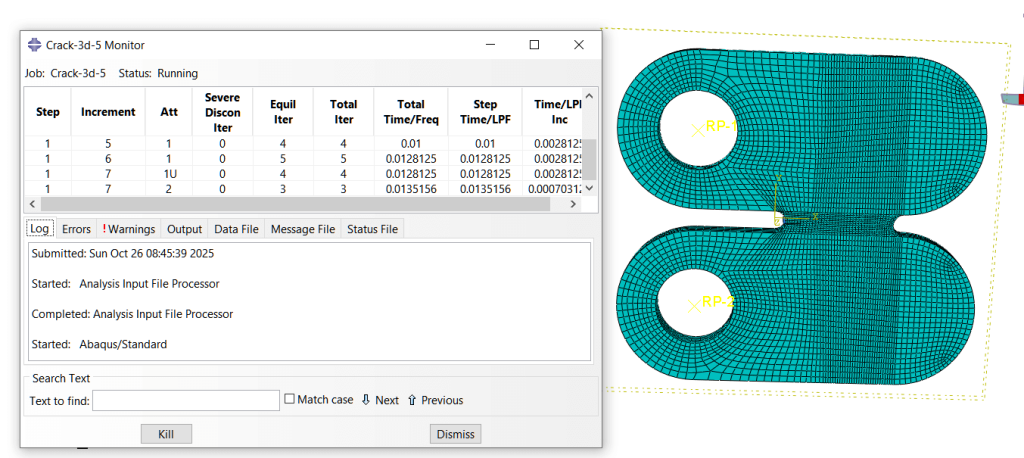
2. Identifying a Convergence Problem: Key Warning Signs
Your Abaqus job will stop prematurely. The Job Manager shows “Aborted” status. This is the first clear sign. The error file provides more details. Check the message file (.msg) carefully. Look for specific error phrases.
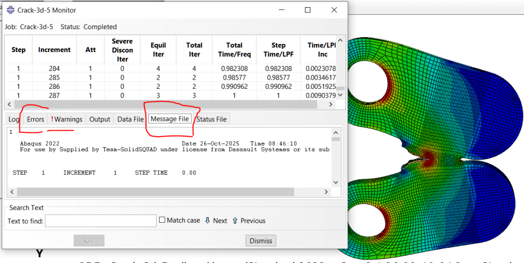
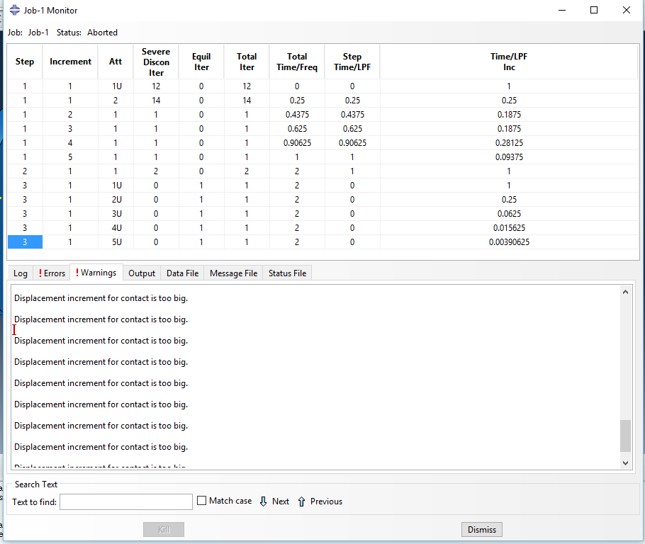
“Too many attempts” appears often. This means the solver tried repeatedly. It could not find equilibrium. “Severe discontinuity” is another common message. This indicates violent contact changes. Forces changed too suddenly.
“Negative eigenvalue” warnings suggest instability. This often means buckling occurred. It can also indicate over-constraint. The time increment becomes very small. It may hit the minimum limit. The analysis cannot move forward.
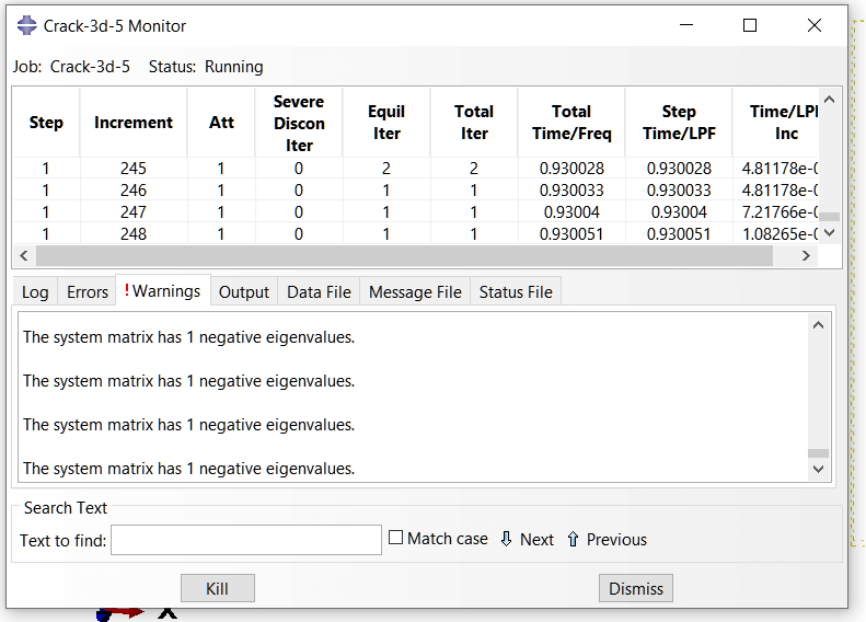
Monitor the job diagnostics while running. Watch the increment number. If it keeps cutting back, trouble is coming. The solution progress stalls completely. These signs help you act fast. You can stop and investigate early.
3. The 10 Major Causes of Convergence Failures
3.1. Non-convergence in a static step (Newton-Raphson)
Typical message (example):**ERROR** THE ANALYSIS HAS NOT CONVERGED - INCREMENT ... FAILED TO CONVERGE
Causes: too large increment, severe nonlinearity, poor load ramp, bad element formulation, unstable contact.
Fixes:
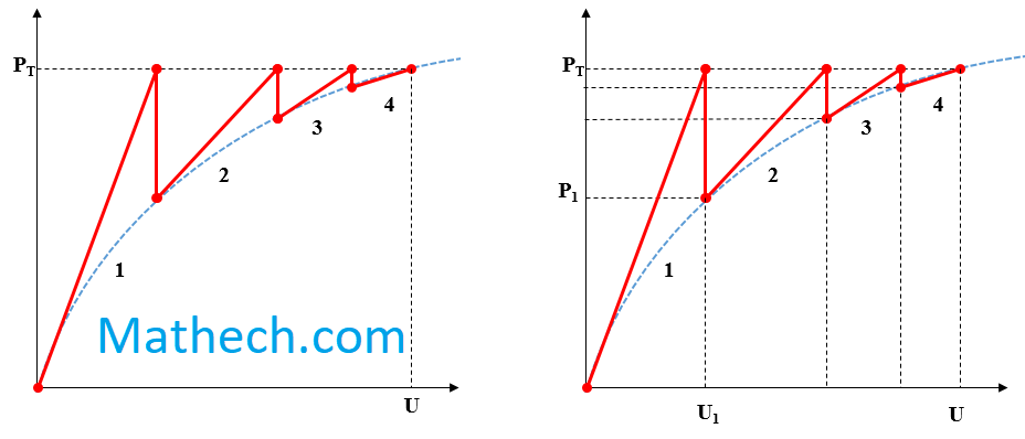
- Reduce initial/time incrementation (Step → Edit → Initial increment / Minimum increment).
- Turn on line search (in GUI: Step → Edit → Solver controls → enable Line search).
- Use
NLGEOM=YESonly when needed (keyword:*STEP, NLGEOM=YES). - Improve mesh or element type (use second-order elements where appropriate).
- Add automatic stabilization: Step → Stabilization (damping factor 1e-4 → increase only if needed).
- If contact: relax contact settings (use penalty with small friction or adjust contact stiffness).
- If all above is done and still no solution, then use:
- *CONTACT CONTROLS, AUTOMATIC TOLERANCES
3.2. Contact non-convergence
Typical messages (examples):WARNING: CONTACT ITERATION DID NOT CONVERGE**ERROR** CONTACT COUPLING FAILED
Causes: poor contact initialization, too-stiff penalty, severe penetration, incompatible surfaces, inappropriate contact algorithm.
Fixes:
- Use Augmented Lagrange or change contact formulation (Surface to surface vs node-to-surface).
- Reduce contact stiffness (Contact → Interaction → edit contact property → reduce stiffness factor).
- Use contact separation/clearance/offset to avoid initial penetration.
- Refine mesh near the contact interface.
- Try small sliding vs finite sliding depending on problem.
- Enable automatic stabilization for contact if oscillatory.
3.3. Element distortion / badly shaped elements
Typical message:WARNING: ELEMENT 12586 HAS BECOME BADLY DISTORTED
Causes: large deformation in single layer of elements, inappropriate element formulation for large strains.
Fixes:
- Refine mesh and improve element aspect ratio.
- Switch to elements better for large deformation (e.g., C3D8R → C3D8I or C3D8R with hourglass control).
- Use remeshing / adaptive meshing (Abaqus/Explicit has ALE or adaptive remesh options).
- Reduce load increment size; use explicit dynamic if implicit cannot handle mesh distortion.
3.4. Material model instability / poor constitutive parameters
Typical message:**WARNING** NON-PHYSICAL MATERIAL RESPONSE DETECTED
(Or solver reports negative stiffness, etc.)
Causes: unrealistic input parameters, abrupt transitions, missing hardening, incorrect units.
Fixes:
- Check units (N, mm vs N, m).
- Smooth the material curve (use small strain vs large strain models appropriately).
- Add viscosity or rate dependence to stabilize (visco-plastic or small viscous regularization).
- For damage models, ensure proper regularization or mesh sensitivity control (use element size / material characteristic length).
- Read more about it : How to deal with excessive element distortion in Abaqus?
3.5. Convergence failure caused by insufficiently small time increments
Typical message:**ERROR** STEP PROGRESS FAILED TO CONVERGE; TIME INCREMENT REDUCED TO MINIMUM
Causes: time increment reduced to minimum but still no convergence.
Fixes:
- Reduce tolerances carefully (change displacement/tolerance thresholds in Step → Solver Controls).
- Increase nonlinear iteration limit (Iterations per increment).
- Use automatic stabilization or replace implicit with explicit if dynamic effects matter.
- Revisit boundary conditions and apply load more gradually (use amplitude curves).
3.6. Rigid body motion / missing boundary conditions
Typical message:**ERROR** RIGID BODY MOTION DETECTED
or many zero pivot messages during matrix factorization.
Causes: model not constrained properly, parts free to translate/rotate.
Fixes:
- Add necessary constraints or reference points.
- Use encastre or pinned BCs for test runs to check model stability.
- For assemblies, use tie constraints correctly, check connector definitions.
3.7. Solver linear algebra issues (singular matrix / zero pivot)
Typical message:**FATAL ERROR** ZERO PIVOT ENCOUNTERED
or **ERROR** MATRIX IS SINGULAR
Causes: disconnected DOFs, duplicate nodes, zero-stiffness elements, bad constraints.
Fixes:
- Run model check: Mesh → Verify mesh connectivity, duplicate nodes removal.
- Check for elements with zero Young’s modulus or zero cross-section area.
- Ensure loads/BCs are not applied to free nodes only.
- Use a small stiffness tie to connect floating parts.
3.8. Explicit solver instability (too large time step / mass scaling side effects)
Typical message:**WARNING** MASS SCALING USED
or energy balance shows KINETIC ENERGY >> INTERNAL ENERGY (sign of instability)
Causes: overly aggressive mass scaling or too-large time step causing non-physical dynamics.
Fixes:
- Reduce mass scaling.
- Refine mesh to reduce critical time increment.
- Use smaller explicit step time or switch to implicit if quasi-static.
- Monitor kinetic vs internal energy to ensure stable dynamic response.
3.9. Convergence issues with nonlinear contact + plasticity
Typical message:**WARNING** LARGE PLASTIC STRAIN CAUSING NONCONVERGENCE
or contact iteration failures while plastic deformation occurs.
Causes: combined geometrical non-linearity and material non-linearity magnify numerical difficulties.
Fixes:
- Ramp load slower (use amplitude curve).
- Use smaller increments and enable line search.
- Use stabilized implicit with viscous regularization on plasticity if available.
- Increase mesh density in plastic zones and use reduced integration cautiously.
3.10. Problems from constraint equations / multi-point constraints (MPC)
Typical message:**ERROR** INCONSISTENT CONSTRAINT EQUATIONS
or solver prints warnings about singularities in constraint matrix.
Causes: conflicting MPCs, overconstrained nodes, incompatible kinematic definitions.
Fixes:
- Check constraint definitions for conflicts (duplicate multipoint constraints).
- Replace MPC with tie or kinematic coupling where appropriate.
- Use rigid body reference nodes instead of many MPCs to simplify constraints.
- Visualize constraint equations to find overlapping constraints.
4. Quick practical checklist to debug any convergence problem
✅ Steps to identify and fix convergence issues
Follow these steps in order to systematically identify and fix convergence issues
Run a linear static check first
If the linear analysis works, then nonlinearity is causing the failure. This helps you isolate the root cause quickly.
Simplify the model
Remove contact interactions, use elastic material properties, and run a small test case to eliminate complexity.
Check units, boundary conditions, and connections
Most convergence problems come from missing constraints, incorrect units, or improper connections between parts.
Refine mesh locally
Mesh refinement near high stress or strain gradients often resolves convergence issues in critical regions.
Read the log files
Check jobname.dat and jobname.msg for iteration details, warning messages, and error codes.
Try different solver controls
Experiment with line search, reduced convergence tolerances, or increase the maximum number of iterations allowed.
Troubleshoot contact problems
If contact repeatedly fails, try surface smoothing, different contact formulations (e.g., penalty vs. augmented Lagrange), or allow small initial gaps.
Final Resort: Try an explicit quasi-static run
If none of the above works, run an explicit analysis with slowly applied loads to get a reference solution. This can help you identify where the standard implicit solver is struggling.
💡 Follow these steps in order. Each step helps narrow down the root cause.
4.1. Notes on exact messages
Abaqus prints many variants. I used typical/representative message text above (examples you will see in .dat, .msg, or on screen). Exact phrasing can vary by version and whether it’s Abaqus/Standard or Abaqus/Explicit. Always check jobname.dat and jobname.log for the precise error lines and the iteration history — those files show the final reason (e.g., which increment failed, element/step numbers, contact pair names).
This guide will show you Overcoming Convergence Issues in Abaqus Welding Simulations
5. Preventing convergence problems before happening
It means building your Abaqus simulations correctly from the start. It focuses on preventing convergence problems before they happen. Instead of fixing errors later, you create stable models initially. You use smart strategies that help the solver work efficiently. This includes proper mesh design and good material definitions.
This guide will show you how to build and mesh a 3D model in Abaqus Learn More
Do not use default increments. They are often too large. Set a small initial increment size. Start with 0.01 or smaller. This helps the solver begin gently. Allow for many increments. Set the maximum to 1000 or more. This gives the solver enough attempts. Also set a small minimum increment. Use 1E-5 or similar. This prevents early termination. Good incrementation guides the solver successfully.
5.1. Increasing increments Strategy: Giving the Solver a Chance
You also set up steps and contacts carefully. These practices make your analysis more reliable. They reduce the risk of failure during solving. This leads to accurate results on the first attempt.
5.2. Stabilization: A Careful Helping Hand
Stabilization helps with tricky models and adds small damping forces. These forces guide the solution. Use automatic stabilization in Abaqus. Set a small dissipation factor. Try 1E-7 initially. Check the energy dissipation later. Ensure it stays below 1-2% of internal energy. Too much stabilization affects results. Remove it once the model works properly.
6. Conclusion: Achieving Reliable Simulation Results
❝ Mastering convergence is essential for successful engineering simulation. By understanding the root causes of failure and implementing systematic solutions, you transform frustrating errors into valuable learning experiences.
✦ Consistent results come from applying proven best practices throughout your modeling process. Remember that patience and methodical troubleshooting always outperform random guessing.
Each solved convergence problem strengthens your FEA expertise and builds confidence in your results. The skills you develop ensure your simulations provide accurate, trustworthy data for engineering decisions.
Continue applying these principles to achieve reliable outcomes project after project.
7. Frequently Asked Questions (FAQ) – Abaqus Convergence Issues
The most common causes of convergence failures in Abaqus include:
1. Material Instabilities: Highly nonlinear material models (e.g., plasticity, hyperelasticity, damage) with poorly defined parameters can cause sudden stiffness changes that the solver cannot handle.
2. Contact Problems: Improper contact definitions, such as insufficient overclosure, incorrect master-slave assignments, or unrealistic friction coefficients, often lead to convergence issues.
3. Mesh Quality: Poorly shaped elements (high aspect ratio, distorted or warped elements) produce inaccurate stress gradients, making it difficult for the solver to reach equilibrium.
4. Large Deformations: Geometrically nonlinear analyses with excessive incremental rotations or strains can cause element distortion and convergence failure.
5. Boundary Conditions: Over-constrained models, rigid body motion, or improperly applied loads can lead to singularities and non-convergence.
6. Time Increment Size: Too large initial or minimum time increments can cause the solver to skip critical nonlinear response regions.
To resolve contact-related convergence issues in Abaqus, consider the following strategies:
1. Adjust Contact Parameters: Use penalty stiffness instead of the default “hard” contact to allow slight penetration, which improves convergence. Reduce the penalty stiffness if oscillations occur.
2. Use Augmented Lagrange Method: This method provides better convergence than pure penalty for frictional contact problems.
3. Refine Contact Definitions: Ensure proper master-slave surface assignment (the stiffer mesh should be the master). Avoid using node-to-surface contact when surface-to-surface is feasible.
4. Smooth Contact Surfaces: Use the *SURFACE BEHAVIOR option with “smooth” contact to avoid sudden changes in contact pressure.
5. Reduce Initial Overclosure: Use the *CONTACT INTERFERENCE option to gradually close gaps over multiple increments rather than solving it in a single increment.
6. Increase the Contact Stiffness Gradually: Use the scale factor feature in *CONTACT CONTROLS to stabilize initial contact.
7. Enable Automatic Stabilization: Use *STABILIZE in contact definitions to add artificial damping that helps overcome convergence difficulties during initial contact.
Mesh quality is critical for convergence because distorted elements produce inaccurate stress and strain gradients, which prevent the solver from reaching equilibrium. Key considerations include:
1. Element Aspect Ratio: Keep the aspect ratio as close to 1.0 as possible. Aspect ratios greater than 10:1 cause significant errors, especially in bending and shear-dominated problems.
2. Element Distortion: Avoid elements with internal angles less than 30° or greater than 150°. Severely distorted elements can cause negative Jacobian determinants, leading to immediate convergence failure.
3. Element Type Selection:
– Use second-order (quadratic) elements for bending-dominated problems (e.g., C3D10, CPE8).
– Use reduced integration elements (C3D8R, CPE4R) for large deformation analyses to avoid shear locking, but be mindful of hourglassing.
– Use hybrid elements for nearly incompressible materials (hyperelasticity, elastoplasticity).
4. Mesh Refinement: Refine the mesh in regions of high stress gradients, contact zones, and near singularities. Use biasing or adaptive meshing to capture local effects.
5. Mesh Convergence Study: Perform a mesh convergence study to ensure the solution is mesh-independent. Refine systematically and monitor convergence of key results (stress, displacement, energy).
6. Avoid Tet Elements in Critical Regions: While tetrahedral elements are convenient, they can exhibit locking. Use hexahedral (brick) elements where possible for better accuracy and convergence.
7. Use Adaptive Mesh Refinement (AMR): In Abaqus/Explicit, use adaptive meshing techniques to handle severe element distortion.
Abaqus offers numerous solver settings and controls to improve convergence. Here are the most effective ones:
1. Load Incrementation:
– Use automatic incrementation with a small initial increment size (e.g., 0.01) to capture nonlinearities gradually.
– Set an appropriate minimum increment size to avoid excessive cuts that waste computational time.
– Use *CONTROLS, PARAMETERS=FIELD to adjust the convergence tolerance for specific field variables.
2. Nonlinear Solution Controls:
– Adjust the line search parameter to help the Newton solver find better equilibrium paths.
– Use automatic stabilization with the *STABILIZE option to add viscous damping in unstable regions.
– Increase the number of equilibrium iterations (default is 12) using *CONTROLS, PARAMETERS=EQUILIBRATION.
3. Contact Controls:
– Use *CONTACT CONTROLS, STABILIZE to add artificial damping during contact transitions.
– Reduce the contact penetration tolerance to avoid excessive overclosure.
4. Mesh Controls:
– Use distortion control in Abaqus/Explicit to prevent element inversion.
– Enable *ADAPTIVE MESH to handle severe distortions in large deformation analyses.
5. Restart and Continue:
– Use restart analysis to continue from a converged increment if the analysis fails. This saves time and helps diagnose the cause of failure.
6. Linear Perturbation:
– For models with initial nonlinearities (e.g., contact prestress, residual stress), perform a linear perturbation analysis first to establish a stable initial state before running the full nonlinear analysis.
7. Diagnostic Output:
– Enable *PRINT, RESIDUAL=YES to print residual forces at each iteration, helping identify problematic regions.
– Use the .msg and .sta files to monitor convergence behavior and identify the root cause of failure.
Preventing convergence failures starts long before you hit the “Submit” button. Follow these best practices to ensure robust analysis:
1. Start Simple:
– Run a linear elastic analysis first to verify mesh, boundary conditions, and load application.
– Gradually add complexity (nonlinear geometry, plasticity, contact, etc.) incrementally to isolate problems.
2. Validate Material Models:
– Test material model parameters on a single-element model first to verify behavior against experimental data or analytical solutions.
– Ensure material parameters are physically meaningful and within applicable ranges.
3. Boundary Conditions:
– Apply minimum necessary constraints to avoid over-constraint while preventing rigid body motion.
– Use smooth loading curves (e.g., ramped amplitude) instead of instantaneous step loading to avoid dynamic effects.
4. Contact Definitions:
– Verify surface normals are correctly oriented for all contact surfaces.
– Use tie constraints for bonded interfaces where no relative motion occurs to improve convergence.
5. Unit Consistency:
– Ensure consistent units throughout the model (length, mass, time, force). Inconsistent units lead to numerical instabilities and convergence failures.
6. Run Diagnostic Checks:
– Use the Data Check run option to detect modeling errors before full analysis.
– Review warning messages in the .dat file and address all warnings.
7. Increment Size Strategy:
– Start with a small initial increment (e.g., 1-5% of the total load/time).
– Set a reasonable minimum increment to prevent excessive cuts that lead to non-convergence.
8. Documentation & Troubleshooting:
– Refer to the Abaqus Analysis User’s Guide Chapter 7 (Convergence) and the Troubleshooting Guide for detailed diagnostics.
– Document each change made to the model to systematically identify what improves convergence.
9. Parallel and Solver Settings:
– Consider using the Direct Sparse Solver instead of the iterative solver for models with highly nonlinear behavior.
– In Abaqus/Standard, enable parallel processing (MPI) to reduce solve times, but ensure your model is well-behaved to avoid parallel-related issues.
10. Training and Experience:
– Understand the physics of your problem—convergence often fails when the model violates physical laws (e.g., unrealistic material behavior).
– Learn from benchmark examples in the Abaqus documentation to understand how similar problems are successfully modeled.
8. Need Expert Help? Solve Your Toughest Convergence Challenges
Is your model still failing? Our Abaqus experts can help. We fix complex convergence issues daily. We save you time and money.