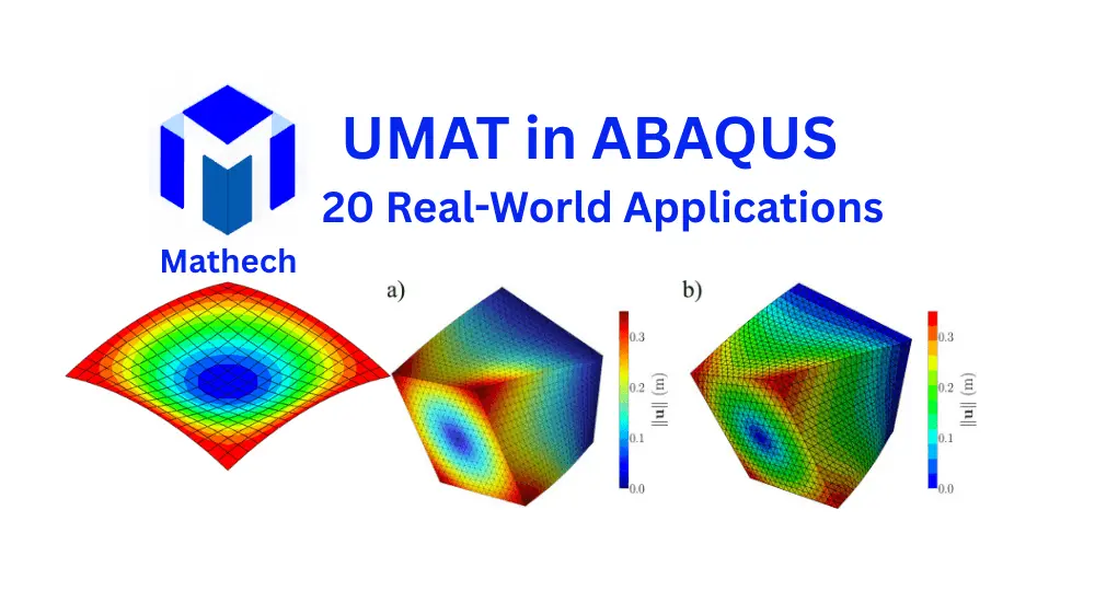
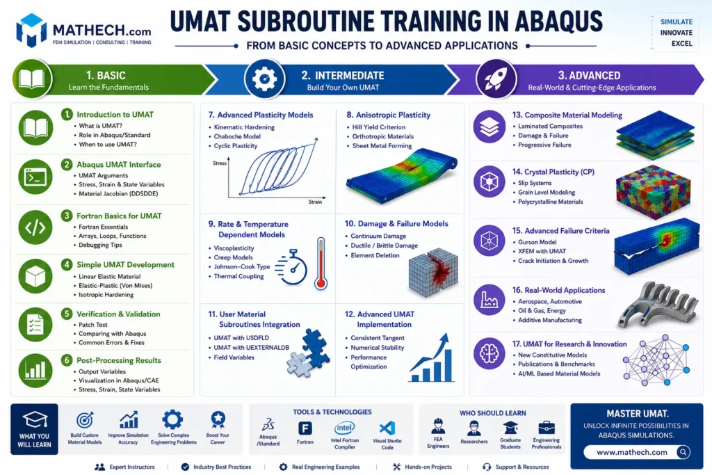
The UMAT subroutine in Abaqus is one of the most powerful tools available for implementing custom material models that extend far beyond the software’s built-in material capabilities. By allowing users to define their own constitutive equations, UMAT enables the accurate simulation of complex material behavior, including plasticity, damage mechanics, creep, composite materials, and other advanced nonlinear phenomena.
In this article, you’ll discover 20 real-world applications of the UMAT subroutine in Abaqus and learn how engineers and researchers use custom material models to solve challenging engineering problems, improve the accuracy of Finite Element Analysis (FEA), and simulate materials that cannot be represented using standard Abaqus models.
📌 What You’ll Discover in This Article
- 20 practical UMAT applications from industry and research
- Where built-in Abaqus material models become insufficient
- Advanced material modeling techniques for nonlinear analysis
- Examples involving metals, composites, polymers, and concrete
- How UMAT improves simulation accuracy and reliability
- Ideas for engineers beginning custom material model development
1. Plasticity Models Beyond Built-in Abaqus Materials
One of the most valuable uses of the UMAT subroutine in Abaqus is the development of custom plasticity models that go beyond the capabilities of the built-in Abaqus material definitions. While Abaqus provides several standard plasticity options, such as isotropic hardening, kinematic hardening, and Johnson-Cook plasticity, many real-world engineering materials exhibit complex behaviors that require more advanced constitutive equations.
1.1. Why Use UMAT for Plasticity Modeling?
Built-in Abaqus plasticity models are suitable for many conventional analyses, but they may not accurately capture:
- Nonlinear hardening behavior observed in metals under large plastic deformation.
- Cyclic loading effects such as ratcheting and the Bauschinger effect.
- Anisotropic yielding in rolled sheets, composites, or textured materials.
- Rate-dependent plasticity where material response changes with strain rate.
- Temperature-dependent yielding in welding, heat treatment, or high-temperature applications.
By implementing a custom plasticity model in UMAT, engineers can define their own stress–strain relationship, hardening law, and state variable evolution to better match experimental data.
1.2. Common Custom Plasticity Models Implemented with UMAT
- Chaboche nonlinear kinematic hardening model for cyclic plasticity and fatigue analysis.
- Hill yield criterion for anisotropic plastic behavior in sheet metal forming.
- Drucker–Prager plasticity extensions for pressure-sensitive materials.
- Modified Johnson–Cook models for high-strain-rate and high-temperature deformation.
- Advanced isotropic/kinematic hardening laws for metals with complex loading histories.
1.3. How UMAT Enhances Plasticity Simulation
In a UMAT implementation, the user typically defines:
- The constitutive equation relating stress increments to strain increments.
- The yield function that determines when plastic deformation begins.
- The hardening rule describing how the yield surface evolves with plastic strain.
- The consistent tangent stiffness matrix, which improves convergence in nonlinear analysis.
- State variables to store internal material history such as plastic strain and back stress.
1.4. Benefits of Custom Plasticity Models
- Higher accuracy in representing material behavior compared to simplified built-in models.
- Better correlation with experiments, especially for cyclic, anisotropic, or high-temperature loading.
- Improved design reliability by predicting permanent deformation and failure more realistically.
- Greater flexibility for implementing new constitutive models from research literature.
Need Expert Abaqus Simulation Support?
Whether you’re facing convergence problems, implementing advanced material models, writing UMAT/VUMAT subroutines, or validating complex finite element analyses, our Abaqus specialists can help you obtain accurate and reliable results.
2. Damage and Failure Modeling
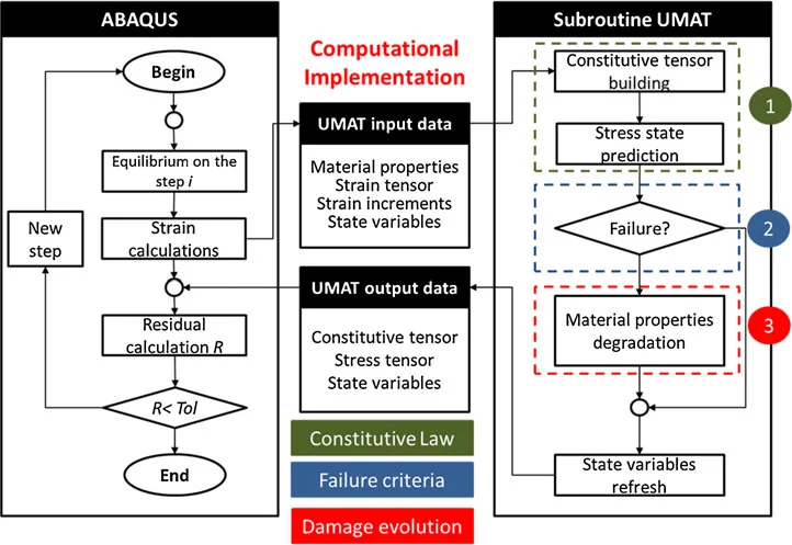
The Abaqus UMAT subroutine enables engineers to implement custom damage and failure models beyond the capabilities of built-in materials. It can simulate stiffness degradation, crack initiation, progressive damage evolution, and material failure under complex loading conditions, making it ideal for composites, metals, concrete, and other advanced engineering materials.
The formulation of a UMAT subroutine for damage and failure modeling in Abaqus is based on developing a user-defined constitutive relationship that describes how a material responds as damage evolves. Unlike built-in Abaqus damage models, UMAT allows researchers and engineers to define custom damage variables, failure criteria, and degradation laws based on experimental observations or advanced theories.
3. Composite Material Modeling
Develop custom constitutive laws for laminated composites and fiber-reinforced polymers.
Common Composite Applications Using UMAT
- Laminated Composites – Modeling ply-by-ply behavior with different orientations.
- Textile Composites – Simulating woven or braided architectures.
- Impact & Crashworthiness – Capturing high-strain-rate failure and energy absorption.
- Fatigue Life Prediction – Implementing cycle-by-cycle damage accumulation.
- Curing & Residual Stress – Simulating manufacturing-induced deformations.
- Sandwich Structures – Modeling core and face-sheet interactions.
- Multiscale Modeling – Bridging micro-scale RVE results to macro-scale structural simulations.
4. Hyperelastic Material Models
Superelastic materials, such as rubber, elastomers, biological tissues, and soft polymers, undergo large elastic deformations and then return to their original shape after unloading. Although Abaqus provides several built-in superelastic models, they may not accurately represent the behavior of newly developed materials or specialized structural laws.
The UMAT subroutine allows engineers to implement custom superelastic formulations based on user-defined strain energy density functions, anisotropic fiber reinforcement, or coupled thermomechanical effects.
During each load increment, UMAT calculates the stress tensor and the corresponding tangent stiffness matrix from the selected strain energy function, ensuring accurate predictions of large strain behavior and strong convergence. This flexibility makes UMAT an essential tool for modeling advanced rubber components, biomedical devices, soft robotics, seals, tires, and other applications involving nonlinear elastic materials.
5. Viscoelastic Material Behavior
Create time-dependent constitutive models for polymers and adhesives.
6. Creep Modeling
Develop custom creep laws for high-temperature components.
Industries
- Power plants
- Turbines
- Pressure vessels
7. Crystal Plasticity
Implement crystal plasticity constitutive models for grain-scale simulations.
Applications
- Single crystals
- Polycrystalline metals
- Additive manufacturing
8. Shape Memory Alloys (SMA)
Model superelasticity and phase transformation behavior.
9. Soil and Geotechnical Materials
Develop advanced constitutive models such as
- Modified Cam Clay
- Bounding Surface Plasticity
- Sand models
10. Concrete Constitutive Models
Implement advanced concrete damage plasticity models beyond Abaqus defaults.
11. Anisotropic Material Models
Model direction-dependent behavior for
- Wood
- Composite materials
- Rolled metals
12. Temperature-Dependent Material Behavior
Couple mechanical properties with temperature evolution.
Applications
- Welding
- Heat treatment
- Fire analysis
13. Phase Transformation Modeling
Simulate transformations such as
- Austenite → Martensite
- Solid-state transformations
14. Functionally Graded Materials (FGMs)
Develop spatially varying material properties.
15. Hydrogen Embrittlement Modeling
Predict degradation caused by hydrogen diffusion.
Industry
- Oil & Gas
- Pipelines
16. Fatigue Damage Accumulation
Implement custom fatigue models that evolve with loading cycles.
17. Biomedical Material Models
Create constitutive laws for
- Bone
- Cartilage
- Soft tissues
- Arteries
18. Smart Materials
Model
- Piezoelectric materials
- Magnetostrictive materials
- Electro-active polymers
19. Additive Manufacturing Material Behavior
Develop constitutive models accounting for
- Layer-wise anisotropy
- Residual stress
- Thermal history
20. User-Defined Constitutive Laws for Research
Implement entirely new constitutive equations published in journals.
Examples include:
- Johnson–Cook modifications
- Gurson-Tvergaard-Needleman (GTN)
- Lemaitre Damage Model
- Chaboche Plasticity
- Hill Yield Criterion
- Drucker–Prager extensions
Frequently Asked Questions in Abaqus UMAT
A UMAT (User MATerial) subroutine is a Fortran-based interface in Abaqus/Standard that allows you to define custom constitutive material models when the built-in Abaqus material library is insufficient. You should use a UMAT when you need to implement advanced mechanical behaviors—such as complex plasticity, creep, damage, or composite failure criteria—that cannot be adequately modeled using standard Abaqus materials. It works at the integration point level, receiving strain increments and returning updated stress and the material Jacobian (tangent stiffness matrix) to the solver for convergence.
To write and run a UMAT, you need three main things:
1. Material model theory: A clear understanding of your material’s constitutive behavior (stress-strain laws, yield functions, hardening rules, etc.).
2. Fortran programming knowledge: UMAT is written in Fortran, so familiarity with the language is essential.
3. A working environment: Abaqus must be properly installed and linked with a Fortran compiler (such as Intel oneAPI). You’ll also need to correctly pass material properties (PROPS) and specify the number of state variables (NSTATV) in the Abaqus/CAE property module.
UMAT subroutines are used across many engineering fields for advanced material modeling. Real-world applications include:
• Concrete structures: Modeling time-dependent creep and shrinkage in prestressed bridges, simulating damage and fracture energy regularization in recycled aggregate concrete, and developing LSTM-based constitutive models for concrete under confining pressure.
• Composites and polymers: Implementing failure criteria like Tsai-Hill for orthotropic composites and using endochronic plasticity theory for short-fiber thermoplastics.
• Fatigue and fracture: Simulating fatigue crack growth acceleration in metals and phase-field modeling of fatigue fracture in porous functionally graded materials.
The main difference is the solver interface and application type:
• UMAT runs with Abaqus/Standard (implicit solver) and is best for static, quasi-static, or slow-loading problems. It requires the user to provide the material Jacobian (DDSDDE) for convergence and is not vectorized.
• VUMAT runs with Abaqus/Explicit (explicit solver) and is ideal for dynamic events like impact, crash, or large deformations. It does not require a Jacobian and is vectorized (processes blocks of integration points at once, using NBLOCK). If your problem involves dynamics or large deformations, you may eventually port your UMAT logic into a VUMAT.
Common challenges include coding errors, memory access violations, incompatible variable dimensions, numerical instabilities, and compiler issues. Here are best practices to avoid them:
• Start simple: Begin with a basic elastic model to test your setup and understand the UMAT structure before adding complexity (plasticity, damage, etc.).
• Debug incrementally: Use PRINT or WRITE statements to catch issues early.
• Double-check dimensions: Ensure variable dimensions (NTENS, NDI, NSHR, NSTATV, etc.) are consistent with your model and Abaqus requirements.
• Provide a consistent Jacobian: For UMAT in Abaqus/Standard, an accurate and consistent DDSDDE matrix is crucial for fast convergence and solver stability. An inaccurate Jacobian can cause slow convergence, divergence errors, or excessive increment cutbacks.