Johnson-Cook Damage Model in Abaqus: Theory and Implementation

The Johnson-Cook (J-C) model is a structural material model. It is widely used to simulate the behavior of metals under high strain rates, large plastic deformations, and high temperatures. In this paper, we will fully explain this model, which is implemented in Abaqus/Explicit software. Based on our experience in finite element simulation, this model is particularly effective for impact analysis, ballistics, and machining simulations.

Show Table of Contents

1. Johnson-Cook Theoretical Foundation

The J-C model, introduced by Johnson and Cook in 1983 , focuses on the characterization of the yield stress and failure strain of materials during deformation. This model takes into consideration three key factors: temperature, strain, and strain rate . It primarily aims to describe the influence of these factors on the material’s behavior, allowing for a better understanding of its mechanical response under varying conditions. By integrating these factors, the J-C model provides a comprehensive understanding of the material’s behavior, allowing for a visualization of the impact of different factors on strain. This enables researchers and practitioners to gain insights into the material’s response to various process conditions and optimize the grinding accordingly.

The J-C model expresses flow stress (σ) as a product of three components:

1.1. Strain Hardening Component

Defines plastic deformation at reference conditions:

σ_hardening = A + Bεⁿ

A: Initial yield stress (MPa)
B: Strain hardening coefficient (MPa)
n: Strain hardening exponent

1.2. Strain Rate Hardening Component

C: Strain rate sensitivity coefficient
ε̇₀: Reference strain rate (s^-1) – Typically 1 s^-1 for metals

1.3. Thermal Softening Component

m: Thermal softening exponent
T_room: Reference temperature (20-25°C)
T_melt: Melting temperature (material’s liquidus temperature)
T_transition: Optional transition temperature threshold

1.4. Damage and Failure Criterion

The Johnson-Cook damage model predicts material failure through damage accumulation:

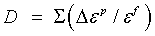
d₁-d₅: Damage parameters (dimensionless)
η: Stress triaxiality (p/q)
ε^f: Equivalent plastic strain at failure
D: Damage variable (failure when D ≥ 1)

2. Material Parameters

Parameter	Description	Typical Units
A	Yield stress at zero strain	MPa
B	Hardening modulus	MPa
n	Hardening exponent	Dimensionless
C	Strain rate coefficient	Dimensionless
m	Thermal softening exponent	Dimensionless
d₁-d₅	Damage model coefficients	Dimensionless
T_melt	Melting temperature	°C
ε̇₀	Reference strain rate	s^-1

Do you want to know our suggested ideas for simulation in Abaqus?

Our experience can help you solve complex finite element simulation problems..

Reach out 100 Project Ideas for Abaqus

3. Defining Johnson-Cook Damage Parameters (d₁-d₅)

3.1 Parameter Significance

The damage parameters d₁-d₅ control material failure prediction in the Johnson-Cook model. These dimensionless coefficients determine how plastic strain accumulates toward failure under different conditions:

Determination Methods

Parameter	Physical Significance	Calibration Method	Typical Range
d₁	Base failure strain at η=0	Uniaxial tension tests	0.01-0.5
d₂	Stress triaxiality sensitivity	Notched specimen tests	0.1-5.0
d₃	Triaxiality exponential factor	Multi-axial loading tests	-3.0-0.0
d₄	Strain rate sensitivity	High-rate testing (SHPB)	0.001-0.1
d₅	Temperature sensitivity	Heated specimen tests	0.0-2.0

3.2 Calibration Process

Experimental Testing:
- Uniaxial tension tests (for d₁)
- Notched specimen tests (for d₂, d₃)
- Split-Hopkinson Pressure Bar (SHPB) tests (for d₄)
- High-temperature tests (for d₅)
Numerical Optimization:
Minimize: Σ(ε_exp^f – ε_model^f)²
Use optimization algorithms to match experimental failure strains

3.3. Johnson-Cook Parameters for AISI 4340 Steel

d₁ = 0.05, d₂ = 3.44, d₃ = -2.12, d₄ = 0.002, d₅ = 0.61

3.4. Abaqus Implementation

*MATERIAL, NAME=STEEL_JC
*JOHNSON COOK DAMAGE
0.05, 3.44, -2.12, 0.002, 0.61
*DAMAGE EVOLUTION, TYPE=DISPLACEMENT
0.1, 0.0001

Where the damage evolution parameters control post-initiation softening

Important Notes

Parameters are highly material-specific
Require validation with multiple test configurations
Negative d₃ values are typical for metals
d₅ > 1 indicates thermal softening accelerates damage

4. Implementation in Abaqus

4.1 Basic Configuration

Define material plasticity using *PLASTIC option
Specify strain rate parameters using *RATE DEPENDENT
Include thermal expansion with *EXPANSION
Define temperature-dependent properties using *DEPVAR

4.2. Advanced Implementation Johnson-Cook suboptions

Johnson-Cook suboptions configuration in Abaqus/Explicit:

*PLASTIC, HARDENING=JOHNSON COOK
*JOHNSON COOK DAMAGE
*DAMAGE EVOLUTION, TYPE=DISPLACEMENT

Plasticity Suboption: Defines strain hardening parameters (A, B, n)
Rate Dependency Suboption: Specifies C and ε̇₀
Damage Initiation: Sets d₁-d₅ parameters
Damage Evolution: Controls post-damage behavior using:
- Linear or exponential softening laws
- Element deletion criteria (D ≥ 1)
- *DAMAGE EVOLUTION parameters for displacement at failure

4.3. Model Limitations

Assumes multiplicative decomposition of effects
Limited accuracy for extreme strain rates (>10⁴ s^-1)
Damage parameters require extensive calibration
Assumes proportional loading for damage accumulation
Limited to isotropic damage representation
Temperature calculation assumes adiabatic conditions

5. Conclusion

The Johnson-Cook model provides an efficient framework for modeling rate-dependent plasticity in Abaqus. Based on our experience, this model is particularly useful for dynamic events in the simulation of the aforementioned cases. Although it has some limitations, its computational efficiency was very interesting and helpful for industrial applications that require the analysis of large deformations. Also, according to the results of various papers, we found that the extension of the damage evolution allows for the prediction of material failure, making it suitable for impact and crash simulation.

You might find these chapters and articles relevant to this topic
Johnson-Cook model

Abaqus Tutorial: Step-by-Step Guide to Simulate Steel Ball Impact on Aluminum Plate

Johnson-Cook Damage Model in Abaqus FAQ – Mathech

6. Frequently Asked Questions (FAQ) – Johnson-Cook Damage Model in Abaqus

What is the Johnson-Cook damage model and what are its key components?

The Johnson-Cook (JC) damage model is a phenomenological material model widely used in Abaqus to simulate ductile fracture in metals subjected to high strain rates, large deformations, and elevated temperatures. It is particularly popular in impact, ballistic penetration, and machining simulations.

The model consists of two main components:

1. Johnson-Cook Plasticity Model (Flow Stress):

Defines the yield stress as a function of plastic strain, strain rate, and temperature.
Equation: σ = [A + B(ε̄^pl)ⁿ] × [1 + C ln(ε̇̄^pl/ε̇₀)] × [1 – (T^*)^m]
A = Initial yield stress at reference conditions.
B = Strain hardening modulus.
n = Strain hardening exponent.
C = Strain rate sensitivity coefficient.
ε̇̄^pl = Equivalent plastic strain rate.
ε̇₀ = Reference strain rate.
T^* = Homologous temperature (normalized by melting temperature).
m = Temperature softening exponent.

2. Johnson-Cook Damage Initiation and Evolution:

Damage Initiation: Defines the equivalent plastic strain at which damage begins, considering stress triaxiality, strain rate, and temperature.
Equation: ε̄_D^pl = [d₁ + d₂ exp(d₃ σ^*)] × [1 + d₄ ln(ε̇̄^pl/ε̇₀)] × [1 + d₅ T^*]
d₁ to d₅ = Damage material constants (typically calibrated from experiments).
σ^* = Stress triaxiality ratio (mean stress / von Mises stress).
Damage Evolution: Defines how material stiffness degrades after damage initiation, typically using a displacement-based or energy-based criterion.

How do I implement the Johnson-Cook damage model in Abaqus?

Implementing the Johnson-Cook damage model in Abaqus is straightforward using the built-in material models. Here is a step-by-step guide:

Step 1: Define Material Properties

Go to the Property module and create a new material.
Set density (if dynamic effects are important).
Define elastic properties (Young’s modulus and Poisson’s ratio).

Step 2: Define Johnson-Cook Plasticity

Navigate to Mechanical > Plasticity > Johnson-Cook Plasticity.
Enter the five material constants: A, B, n, C, and m.
Define reference strain rate (ε̇₀) and melting temperature (T_melt).
Specify the transition temperature (T_transition) if needed.

Step 3: Define Johnson-Cook Damage Initiation

Navigate to Mechanical > Damage for Ductile Metals > Johnson-Cook Damage Initiation.
Enter the five damage constants: d₁, d₂, d₃, d₄, and d₅.
Specify the reference strain rate (often same as plasticity reference).
Set the temperature dependencies if applicable.

Step 4: Define Damage Evolution

Navigate to Mechanical > Damage for Ductile Metals > Damage Evolution.
Choose Type: Displacement or Energy.
Specify fracture energy or effective plastic displacement at failure.
Set degradation options (linear or exponential softening).

Step 5: Define Element Deletion

In the Damage Evolution options, set Element Deletion to “Yes”.
Specify the maximum degradation threshold (typically 0.99 or 1.0).

Step 6: Mesh and Analysis Setup

Assign the material to your sections.
Use fine mesh in regions where damage is expected.
Consider using explicit dynamics (Abaqus/Explicit) for high-strain-rate applications.

Step 7: Validate the Model

Run a single-element test to verify the material response.
Compare with experimental data (tensile, torsion, or Hopkinson bar tests).
Calibrate constants if necessary using optimization tools.

How do I calibrate the Johnson-Cook damage model parameters for my material?

Calibrating the Johnson-Cook damage model parameters is a critical step that requires experimental data and systematic fitting. Follow this comprehensive calibration procedure:

Step 1: Collect Experimental Data

Quasi-static tensile tests at different temperatures (e.g., -40°C, 25°C, 200°C, 500°C).
Dynamic tests using Split Hopkinson Pressure Bar (SHPB) at various strain rates (10²–10⁴ s⁻¹).
Torsion tests to capture large strain behavior up to fracture.
Notched tensile tests with different notch geometries to vary stress triaxiality.

Step 2: Calibrate Plasticity Parameters (A, B, n, C, m)

Fit A, B, n from quasi-static tensile data at room temperature.
Fit C from dynamic test data (plot yield stress vs. log strain rate).
Fit m from temperature-dependent test data (plot yield stress vs. temperature).
Use curve fitting tools (MATLAB, Python, or Excel) to find best-fit values.
Validate the model against independent data sets not used for fitting.

Step 3: Calibrate Damage Parameters (d₁, d₂, d₃, d₄, d₅)

d₁, d₂, d₃ (triaxiality dependence) are calibrated from tests at different stress triaxialities.
d₄ (strain rate dependence) is calibrated from dynamic tests at various strain rates.
d₅ (temperature dependence) is calibrated from tests at different temperatures.
Perform fracture strain measurements from post-test specimens.
Use inverse modeling (simulate test and match force-displacement curves).

Step 4: Calibrate Damage Evolution

Determine fracture energy from load-displacement curves (area under the curve).
Calculate effective plastic displacement at failure from simulation of standard tests.
Adjust softening behavior (linear vs. exponential) based on experimental observations.

Step 5: Practical Tips for Calibration

Start with published parameters for similar materials as initial guesses.
Use optimization algorithms (genetic algorithms, gradient-based) for multiple parameters.
Validate the model with independent test cases (e.g., different specimen geometries).
Document all experimental conditions (strain rate, temperature, specimen dimensions).
Consider uncertainty quantification to assess parameter sensitivity.

What are the common convergence issues with the Johnson-Cook damage model and how can I resolve them?

The Johnson-Cook damage model can cause significant convergence difficulties due to the sudden material softening and element deletion. Here are common issues and solutions:

1. Convergence Issues in Abaqus/Standard

Problem: Sudden element deletion creates unbalanced forces and convergence failure.
Solution: Use viscous regularization (add small viscosity coefficient to damage evolution).
Solution: Reduce element size in damage zones to allow gradual energy dissipation.
Solution: Use small initial increment sizes to capture softening gradually.
Solution: Consider switching to Abaqus/Explicit for highly unstable problems.

2. Mesh Sensitivity Issues

Problem: Results depend on element size because damage evolution is mesh-dependent.
Solution: Use energy-based damage evolution (fracture energy) instead of displacement-based.
Solution: Maintain consistent mesh refinement across the damage zone.
Solution: Use regularized damage models with length-scale dependency.

3. Element Distortion in Explicit Analyses

Problem: Severely distorted elements cause negative Jacobian and simulation crashes.
Solution: Use hourglass control (enhanced or stiffness) to prevent excessive distortion.
Solution: Implement adaptive meshing (ALE) to handle large deformations.
Solution: Reduce time increment size (CFL condition) to maintain stability.

4. Premature Element Deletion

Problem: Elements delete too early, causing unrealistic fracture patterns.
Solution: Increase the damage threshold (maximum degradation before deletion).
Solution: Use status variable to control deletion more precisely.
Solution: Calibrate damage evolution parameters more accurately.

5. Material Instability

Problem: Negative tangent stiffness causes non-convergence.
Solution: Add artificial viscosity in the material definition.
Solution: Use stabilization (automatic or manual) in contact definitions.
Solution: Reduce the strain rate sensitivity parameter (C) if overly stiff.

6. General Troubleshooting Tips

Run Data Check to identify issues before full analysis.
Monitor .msg and .sta files for convergence warnings.
Use single-element tests to debug material behavior independently.
Implement incremental loading to control damage progression.
Consider two-step analysis: first without damage to establish state, then with damage.

What are the best practices and common applications for the Johnson-Cook damage model?

To achieve accurate and reliable results with the Johnson-Cook damage model, follow these best practices and understand its common applications:

Best Practices:

Validate extensively: Always validate model predictions against experimental data for multiple loading conditions.
Use appropriate element types: Use reduced integration elements with hourglass control (C3D8R, CPE4R) for efficiency.
Maintain mesh quality: Use fine, regular mesh in damage zones with aspect ratios close to 1.
Select correct solver: Use Abaqus/Explicit for high-strain-rate and highly nonlinear analyses.
Define material units consistently: Use consistent units for stress, strain, and energy.
Perform sensitivity analysis: Assess the effect of each parameter on model predictions.
Document all parameters: Record material constants, reference conditions, and calibration procedures.
Use temperature-dependent properties: Include thermal effects for applications involving significant heating.

Common Applications:

Ballistic Impact and Penetration: Simulating bullet or fragment penetration into metallic armor and structures.
Metal Machining and Cutting: Modeling chip formation, tool wear, and surface integrity in machining operations.
High-Speed Forming: Analyzing explosive forming, electromagnetic forming, and other high-rate deformation processes.
Aerospace Structures: Simulating bird strikes, foreign object damage (FOD), and crashworthiness of aircraft components.
Automotive Crashworthiness: Predicting vehicle component failure during collisions and crash scenarios.
Manufacturing Processes: Modeling forging, extrusion, and rolling processes with high strain rates.
Fracture Mechanics: Analyzing ductile fracture initiation and propagation in structural components.
Mining and Drilling: Simulating rock cutting and drilling operations with high-speed impacts.
Nuclear Applications: Modeling fuel rod cladding behavior under accident conditions.
Defense and Armor Design: Optimizing armor systems against various projectile threats.

Additional Recommendations:

Study compatibility: The Johnson-Cook model is available in both Abaqus/Standard and Abaqus/Explicit.
Combine with other models: Can be coupled with progressive damage or cohesive zone models.
Consider thermal effects: Include thermal conductivity and specific heat if temperature rise is significant.
Use material user subroutine (UMAT/VUMAT): For custom modifications to the Johnson-Cook model.
Consult literature: Review published Johnson-Cook parameters for common materials (e.g., steel, aluminum, titanium, copper).

Johnson-Cook Damage Model in Abaqus: Theory and Implementation