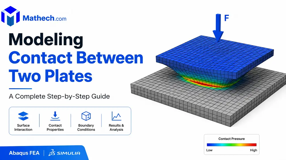
Contact simulations in Abaqus require accurate representation of the interaction between surfaces, especially when the objective is to predict contact pressure distribution and load transfer between components. In this study, the mechanical interaction between two plates is analyzed under an applied vertical load to determine the contact pressure developed at the interface.
Engineering Problem Definition and Contact Analysis Objectives
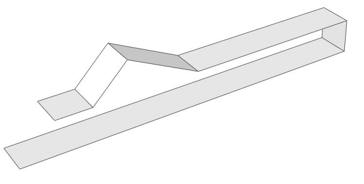
The model consists of an upper and lower plate that initially interact through a contact interface. A prescribed displacement is applied to the upper plate, causing deformation and contact pressure generation between the two surfaces. The primary output of interest is the contact pressure distribution (CPRESS) along the contact region.
The original problem investigates the contact behavior between two plates subjected to a linear load, where the contact pressure between surfaces must be extracted from the Abaqus simulation results.
Choosing Between Shell and Solid Modeling Approaches
For relatively thin plates where through-thickness deformation is not the primary concern, shell elements can provide efficient results with lower computational cost. In the presented model, the plates are represented using shell geometry, reducing the computational effort while maintaining sufficient accuracy for contact pressure evaluation. This workflow defines the model as a deformable shell extrusion in Abaqus.
However, solid elements should be considered when:
- Significant thickness deformation occurs.
- Contact pressure varies through the thickness.
- Plastic deformation develops near the contact region.
- Detailed stress gradients are required.
For industrial contact problems, the modeling strategy should balance computational efficiency and physical accuracy.
Step 1: Creating the Plate Geometry in Abaqus
Defining the Upper and Lower Plate Geometry
The reference model uses a 3D deformable shell extrusion approach.
Begin by entering the Part module and clicking on Create Part. In the dialog box that appears, configure the following settings:
- Modeling Space: 3D
- Type: Deformable
- Base Feature: Shell
- Approximate Size: 50
Click Continue to proceed.
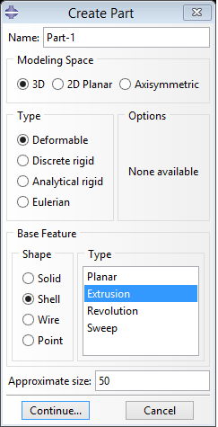
This step establishes the fundamental geometry of your plates as 3D deformable shell features.
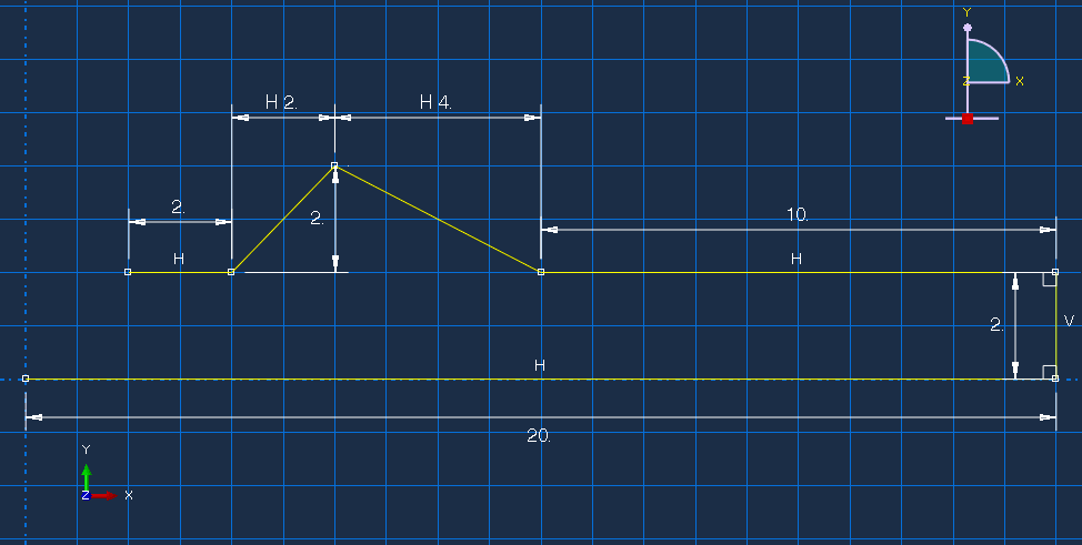
Key Considerations for Contact Geometry Creation
When creating contact geometries, several aspects must be considered:
- The contacting surfaces must be clearly defined.
- Sharp geometric discontinuities should be avoided unless physically required.
- The initial gap or penetration between surfaces must be controlled.
- The geometry must allow realistic deformation under applied loading.
Incorrect initial positioning can create artificial penetration, excessive initial contact forces, or convergence difficulties during analysis.
Step 2: Defining Material Properties
Assigning Linear Elastic Material Behavior
The mechanical response of the plates is defined through the material module. For this simulation, an elastic material model is used with Young’s modulus and Poisson’s ratio as the required parameters.
Navigate to the Property module and double-click on Material in the model tree. Define the mechanical properties as follows:
- Mechanical → Elasticity
- Young’s Modulus: 210,000 MPa
- Poisson’s Ratio: 0.3
Click OK to save the material definition.
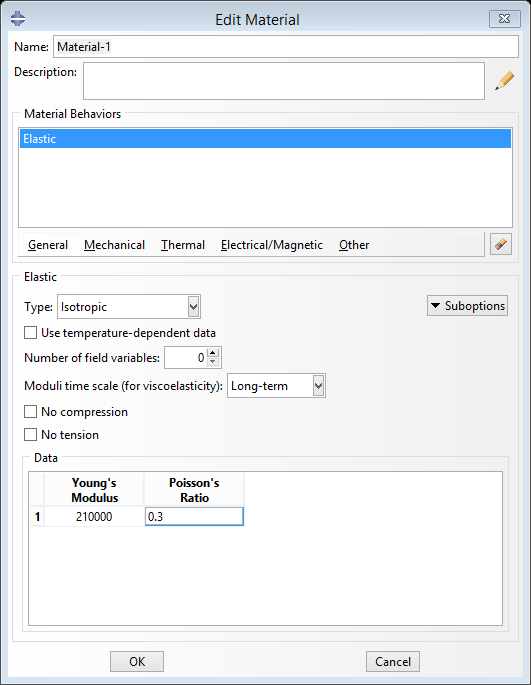
These properties represent a typical metallic material behavior.
Key Considerations for advanced contact simulations
For more advanced contact simulations, the material model should be selected based on the expected loading condition. Linear elasticity is suitable when:
- Stresses remain below yield strength.
- Permanent deformation is negligible.
- Contact forces are moderate.
For applications involving high contact pressure, such as metal forming, wear, or impact problems, plasticity models may be required.
Step 3: Creating and Assigning Sections
Selecting the Appropriate Shell Section
After defining the material behavior, the section properties are created and assigned to the plate geometry.
The reference model uses a homogeneous shell section with a defined thickness value.
Section assignment ensures that the Abaqus solver has access to:
- Material properties.
- Thickness information.
- Element formulation requirements.
The section must be assigned to the complete model region before continuing to assembly creation.
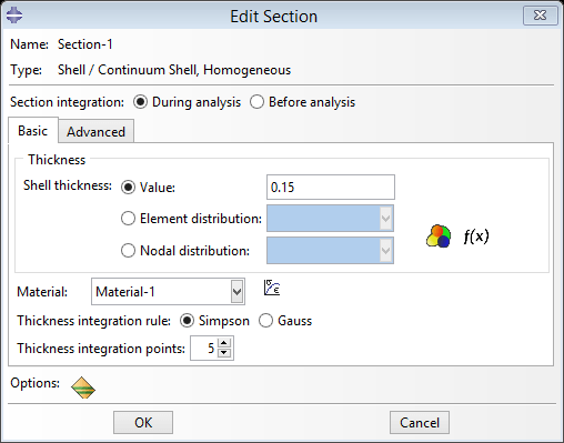
Create Section
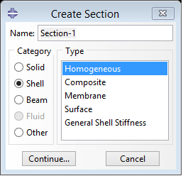
Click on the Create Section icon. In the dialog box, select:
- Category: Shell
- Type: Homogeneous
Click Continue. In the next window, set the shell thickness to 0.15 and click OK.
Step 4: Assign Section to the Part
Click on the Assign Section icon and select the entire model. In the dialog box, choose Section-1 and click OK.
Note: After successfully assigning the material and section, the entire model will turn green, confirming proper assignment.
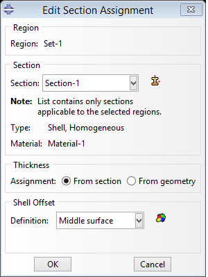
This step links your material properties and section definition to the actual geometry.
Defining a section assigns physical characteristics (like thickness) to your shell geometry
Incorrect section assignment is one of the common causes of inaccurate deformation predictions because Abaqus cannot correctly calculate stiffness without proper material and thickness definitions.
Step 5: Create the Assembly Instance
Creating Independent Instances
After completing the individual parts, the geometry is transferred into the Assembly module.
Enter the Assembly module. In the model tree, double-click on Instance under the Assembly branch. Accept the default settings in the dialog box and click OK.
Creating an instance allows you to position your part within the global coordinate system for analysis.
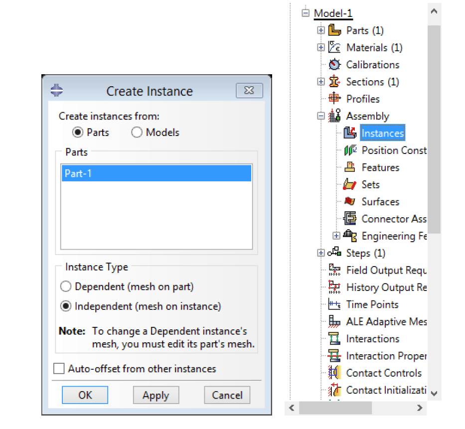
The plates are inserted as independent instances, allowing Abaqus to treat each component separately during contact calculations.
Independent instances are useful when:
- Components may deform independently.
- Contact occurs between separate bodies.
- Different boundary conditions are applied to each component.
Before defining contact interactions, the relative position of both plates should be verified carefully. The initial configuration determines whether the contact surfaces begin separated or already engaged.
Step 6: Configuring the Static Analysis Step
Creating a Static General Step
The contact problem is solved using the Static General procedure available in Abaqus/Standard. This step is appropriate for slowly applied mechanical loading where inertial effects are negligible.
See more Choosing Appropriate Analysis Procedures in Abaqus
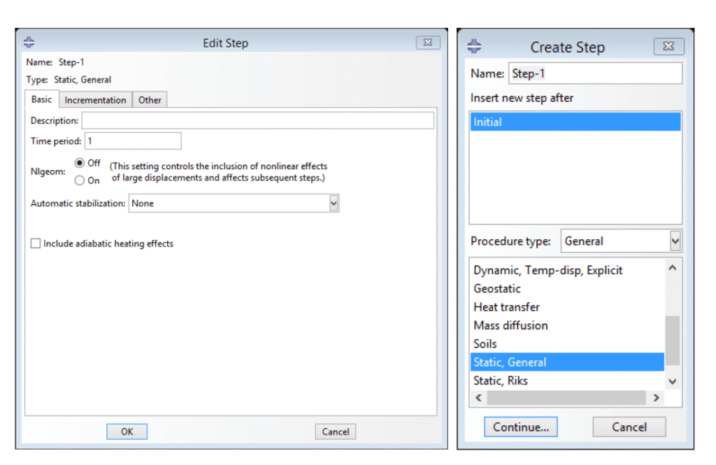
The reference model creates a General Static step with default settings.
Although default settings may work for simple cases, complex contact simulations often require adjustment of:
- Initial increment size.
- Maximum increment number.
- Automatic stabilization.
- Contact controls.
Contact problems are inherently nonlinear because the contact area changes during loading. Therefore, appropriate increment control is essential for maintaining convergence.
Step 7: Applying Boundary Conditions
Preventing Rigid Body Motion
Boundary conditions define how the plates are constrained during loading. The fixed plate must be restricted sufficiently to prevent rigid body movement while avoiding unrealistic constraints.
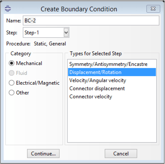
Create boundary conditions by clicking on Create Boundary Condition:
- Step: Initial
- Category: Mechanical
- Types: Symmetry/Antisymmetry/Encastre
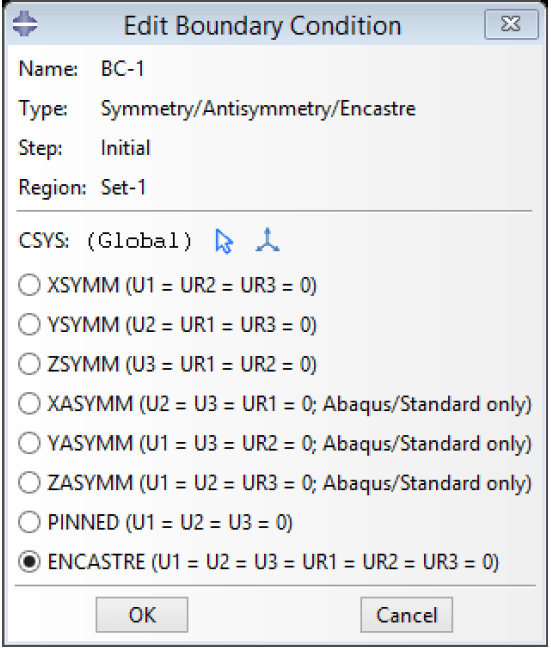
Click Continue and select the appropriate edges/faces for fixing.
Boundary conditions constrain the model to simulate realistic support conditions for the plates
The reference model applies an encastre boundary condition to constrain the selected region.
A correct constraint strategy should:
- Represent the real physical support.
- Remove unnecessary degrees of freedom.
- Avoid artificial stress concentrations.
Over-constraining the model can significantly alter contact pressure results and produce unrealistic reaction forces.
Step 8: Define Displacement Loading
Create another boundary condition by clicking Create BCs again:
- Step: Step-1
- Category: Mechanical
- Types: Displacement/Rotation
Click Continue, select the line shown in the diagram, and set the displacement value to 2 mm in the specified direction. Click OK.
This applies the linear load through prescribed displacement on the top plate.
Step 9: Define Contact Properties
Creating Contact Interaction Properties
The accuracy of a contact simulation depends primarily on how the interaction between the two surfaces is defined. In Abaqus, this begins by creating a contact property that controls both the normal and tangential behavior of the interface. The reference workflow creates a contact interaction property in the Interaction module before assigning it to the contacting surfaces.
Two fundamental behaviors must be specified:
- Normal behavior, which controls how the surfaces resist penetration.
- Tangential behavior, which defines frictional resistance during sliding.
Selecting inappropriate contact properties is one of the most common reasons for poor convergence and unrealistic contact pressure predictions.
Configuring Normal Contact Behavior
For this example, the normal contact behavior uses Hard Contact with the Penalty enforcement method because the plates are initially separated before loading. The penalty formulation allows a small numerical penetration while maintaining stable convergence in most static contact analyses.
Alternative formulations, such as augmented Lagrange or direct constraint methods, may improve contact accuracy for highly nonlinear problems but often require tighter convergence controls and additional computational effort.
Configuring Tangential Contact Behavior
The reference model assumes frictionless contact, eliminating tangential resistance between the plates.
This assumption is appropriate when:
- Lubricated interfaces are analyzed.
- The objective is to evaluate only normal contact pressure.
- Sliding resistance has a negligible influence on the structural response.
For engineering applications involving dry metal contact, a Coulomb friction model should be considered. Typical friction coefficients range from 0.1 to 0.3 depending on surface finish, lubrication, and material combination.
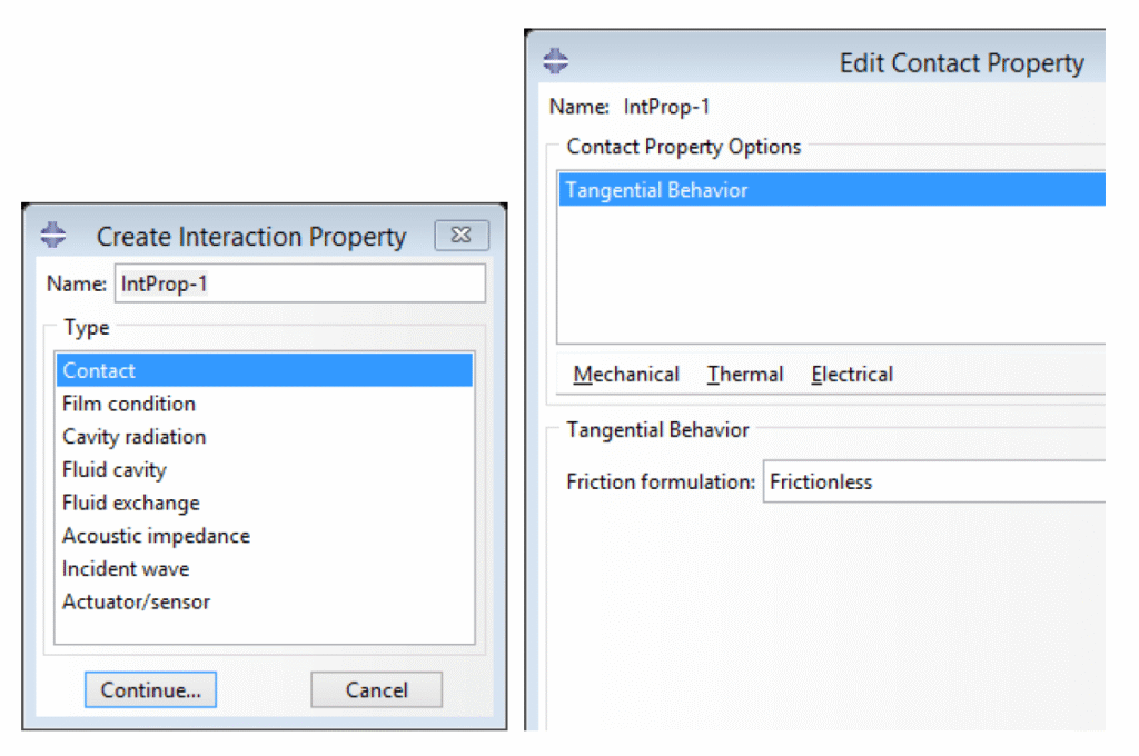
Create Interaction Properties
Enter the Interaction module and click on Create Interaction Properties. Select:
- Contact as the interaction type
- Click Continue
In the new window, go to the Mechanical tab and select Tangential Behavior with Frictionless contact.
Defining contact properties establishes how the two plates interact when they come into contact.
Step 10: Create Contact Interaction
Selecting Master and Slave Surfaces
After defining the contact property, the interacting surfaces are assigned as Master and Slave. The tutorial selects the lower plate as the master surface and the upper plate as the slave surface.
As a general guideline:
- The stiffer or coarser mesh should be selected as the master surface.
- The finer mesh should be assigned as the slave surface.
- Contact surfaces should have compatible discretization to reduce numerical noise.
Incorrect master-slave selection can lead to excessive penetration, unstable contact pressure, and convergence issues.
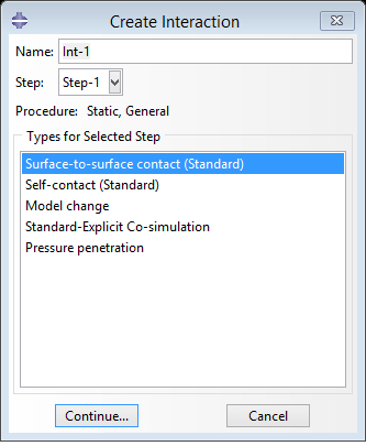
After defining contact properties, click on Create Interaction:
- Select Surface to Surface Contact
- Click Continue
Select the lower surface as the Master Surface (shown in purple in the diagram). Note that the purple surface contacts the upper plate.
Proper master-slave surface selection is crucial for accurate contact simulation convergence.
Step 11: Mesh Strategy for Contact Analysis in Abaqus
Selecting Appropriate Element Size
Mesh quality strongly influences the accuracy of contact pressure calculations. Since contact stresses vary rapidly near the interface, coarse meshes may significantly underestimate peak pressures.
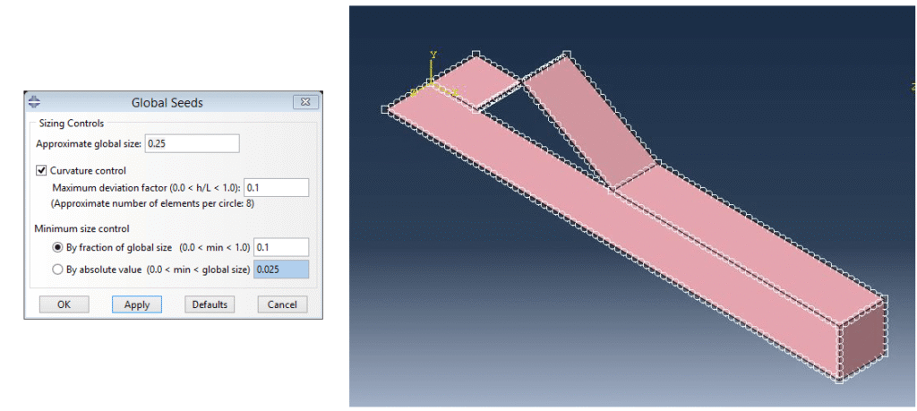
The reference workflow applies a global mesh seed before generating the mesh.
For industrial simulations, engineers often use:
- A coarse mesh away from the contact region.
- Local refinement at the contact interface.
- Smooth mesh transitions to minimize stiffness discontinuities.
Enter the Mesh module and click on the Global Seeds icon. In the dialog box, set the global seed size to 0.25 and click OK. Then generate the mesh.
This strategy improves solution accuracy while keeping computational cost under control.
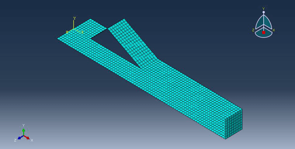
Choosing the Element Type
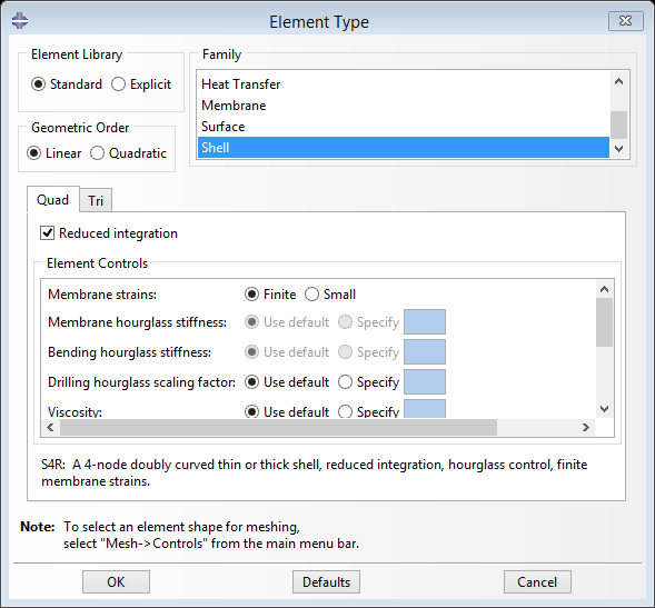
After meshing, the element formulation is assigned. The tutorial uses shell elements appropriate for thin plate structures.
When selecting elements for contact simulations, consider:
- Reduced integration elements for computational efficiency.
- Higher-order elements when stress gradients are significant.
- Compatible element formulations for both contacting bodies.
Element distortion should also be monitored because poor-quality elements reduce contact accuracy and solver robustness.
A finer mesh density at the contact interface typically yields more accurate contact pressure results.
Step 12: Submit the Job for Analysis
Creating and Executing the Analysis
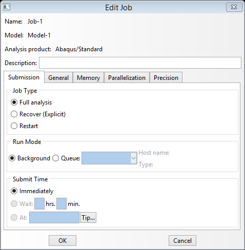
Once preprocessing is complete, the model is submitted through the Job module. The workflow creates a new job using the default analysis settings before submitting it for solution.
Before launching the simulation, engineers should verify:
- Missing section assignments.
- Undefined material properties.
- Contact pair definitions.
- Boundary conditions.
- Mesh quality.
- Analysis step configuration.
A preliminary model check can eliminate many errors before the solver begins the nonlinear iterations.
Creat Job
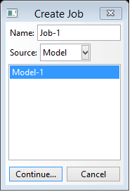
Enter the Job module and click on Create Job:
- Name: Job-1
- Click Continue, then OK
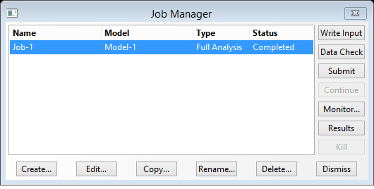
From the Job Manager, click Submit to start the analysis.
This step sends your complete model to the Abaqus solver for finite element analysis.
Step 12: Post-Processing Contact Results
Evaluating Contact Pressure (CPRESS)
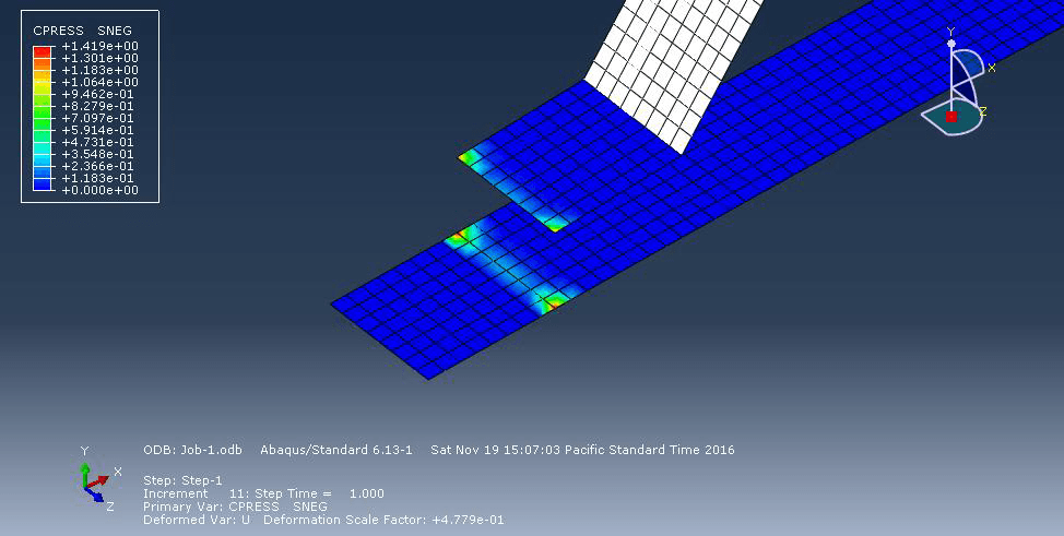
The primary objective of this analysis is to determine the contact pressure distribution between the two plates. After the analysis completes successfully, Abaqus displays the deformed shape and field output results in the Visualization module. The tutorial recommends plotting the CPRESS output variable to visualize the pressure distribution across the contact interface.
High contact pressure regions typically indicate:
- Localized load transfer.
- Stress concentration.
- Potential wear locations.
- Risk of yielding or surface damage.
CPRESS should always be interpreted together with the contact area rather than considering only the peak pressure value.
After the analysis completes successfully (you’ll see a “Completed” message in the Job Manager), click Results to enter the Visualization module.
View Results
To view results:
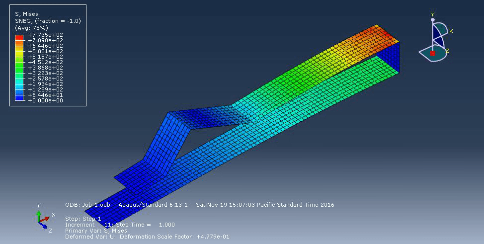
- Click Plot Contours on Deformed Shape to see deformation patterns
- From the Field Output toolbar, select CPRESS to view contact pressure distribution between the two surfaces
Visualizing CPRESS (Contact Pressure) allows you to examine the stress distribution at the plate interface, which is the primary objective of this analysis.
Additional Results to Review
Although contact pressure is the primary result, a comprehensive evaluation should also include:
- Total deformation.
- Von Mises stress.
- Contact status.
- Reaction forces.
- Contact opening and closing behavior.
Comparing these outputs provides a more complete understanding of structural performance under loading.
Validating the Contact Simulation
Numerical results should never be accepted without verification. A reliable validation process includes:
- Performing a mesh convergence study.
- Confirming reaction force equilibrium.
- Checking that contact pressure varies smoothly.
- Comparing numerical predictions with analytical solutions or experimental measurements whenever available.
Validation is particularly important for engineering designs where contact pressure influences fatigue life, wear, or structural safety.
Common Modeling Errors
Several common mistakes can significantly reduce simulation accuracy:
- Assigning the wrong master and slave surfaces.
- Using an excessively coarse mesh near the contact interface.
- Applying unrealistic boundary conditions.
- Defining incorrect contact properties.
- Allowing initial geometric penetration between contacting bodies.
- Applying large displacement increments that prevent convergence.
Most convergence problems originate from preprocessing decisions rather than limitations of the solver itself.
Best Practices and Engineering Recommendations
For reliable plate contact simulations in Abaqus:
- Refine the mesh only where contact stresses are expected.
- Select contact formulations that match the physical problem.
- Apply displacement-controlled loading whenever possible for improved convergence.
- Verify boundary conditions before each analysis.
- Validate the model using mesh sensitivity studies and available experimental data.
- Review multiple output variables instead of relying solely on CPRESS.
Following these practices produces more accurate and computationally efficient simulations while reducing the likelihood of convergence issues.
Conclusion
Modeling contact between two plates in Abaqus requires more than simply defining two interacting surfaces. Accurate predictions depend on appropriate geometry representation, material definition, contact formulation, mesh refinement, boundary conditions, and solver configuration. By combining a robust preprocessing workflow with careful validation and interpretation of CPRESS results, engineers can confidently evaluate load transfer, identify critical contact regions, and improve the reliability f structural designs. The workflow presented in the reference tutorial provides a solid foundation for static contact analysis and can be extended to more advanced applications involving friction, plastic deformation, or complex multi-body assemblies