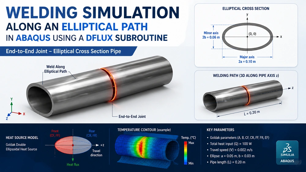
Moving-heat-source welding simulation is one of the most powerful capabilities in Abaqus for predicting residual stress, distortion, and the thermal history of welded components. Most tutorials demonstrate a heat source traveling in a straight line or a circle, because those paths are easy to parameterize. Real fabrication, however, often follows more complex geometries- flanges, nozzle attachments, and sealing welds that trace an ellipse.
An elliptical weld path introduces a subtlety that trips up many engineers: the torch does not move at a constant angular rate. If you naively write angle = ω·t, the heat source will race through the sharply curved ends of the ellipse and crawl along the flatter sides, giving you the wrong heat input per unit length and an unphysical weld pool.
This article explains the correct formulation and provides a complete, tested DFLUX subroutine that keeps the travel speed constant along an ellipse.
Why an Ellipse Is Not Just a Stretched Circle
For a circle of radius R, arc length and angle are proportional: . Move at angular speed ω=v/R and the linear speed is automatically constant.
For an ellipse with semi-axes and , the position is:
The speed at which the point travels as increases is the magnitude of the derivative:
This quantity changes with position — it equals be at the ends of the major axis and ae along the minor axis. Because there is no closed-form inverse of the elliptic arc-length integral, we must handle it numerically.
The physical requirement is a constant travel speed , so the arc length covered must satisfy:
The simulation therefore has to:
- Compute the total perimeter of the ellipse.
- Convert the current analysis time into an arc length, .
- Invert to recover the parametric angle .
- Build a local weld frame (travel direction + transverse + depth) at that point.
- Evaluate the Goldak double-ellipsoid flux.
Abaqus DFLUX Workflow for a Moving Heat Source on an Elliptical Weld Path
How the Fortran subroutine keeps the torch at constant travel speed around an ellipse using arc-length parameterisation, then applies the Goldak double-ellipsoid heat distribution at every integration point.
Initialise flux and validate the load type
Zero the flux on every call and exit unless Abaqus is requesting a body flux, so unrelated load types are never overwritten.
FLUX(1) = 0.D0
IF (JLTYP .NE. 1) RETURNDeclare path, source and process parameters
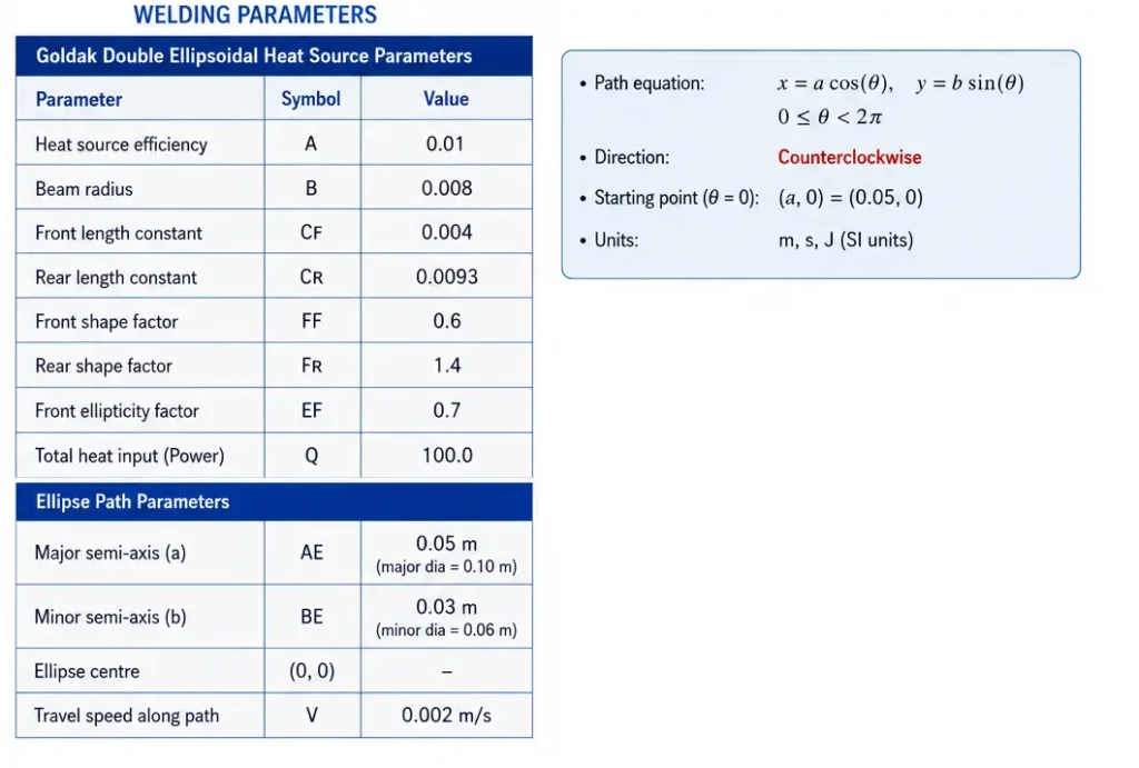
Ellipse semi-axes, Goldak ellipsoid dimensions, arc power, efficiency and travel speed are set in one place for easy calibration.
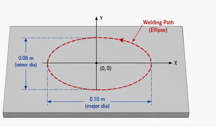
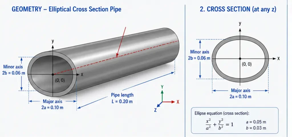
ae = 0.05 m, be = 0.03 m (major Ø 0.1 m, minor Ø 0.06 m)
Q = 1218 W, η = 0.7, a = 0.010, b = 0.008, cf = 0.004, cr = 0.0093
ff = 0.6, fr = 1.4, v = 0.002 m/sCompute the ellipse perimeter by Simpson integration
An ellipse has no closed-form perimeter, so the arc-length integrand is integrated over 0 to 2π with N = 720 panels.
P = ∫02π √( ae² sin²θ + be² cos²θ ) dθ ≈ 0.2549 mConvert analysis time to travelled distance
Distance grows linearly with time at the prescribed travel speed, then wraps within one perimeter so multi-pass circumferential welds continue seamlessly.
S = v · t → S = S − P · ⌊S / P⌋ (one lap ≈ 127.4 s)Invert arc length to parametric angle
Constant angular velocity would give a variable travel speed on an ellipse, so s(θ) is inverted numerically: march through sub-arcs to bracket S, then refine with Newton–Raphson.
θk+1 = θk + ( S − s(θk) ) / |r′(θk)| (≤ 20 iterations)Locate the source centre and build the local weld frame
Place the torch on the ellipse, then form the unit tangent (travel direction) and unit normal (transverse direction) at that point.
yc = ae cos θ, zc = be sin θ
t = (−ae sin θ, be cos θ) / |r′| n = (be cos θ, ae sin θ) / |r′|Project the integration point into Goldak coordinates
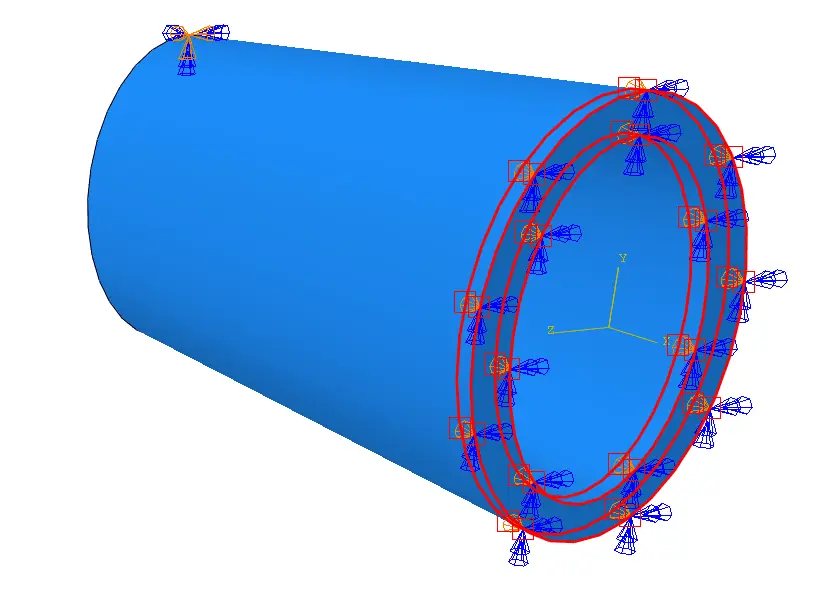
The offset between COORDS and the source centre is projected onto the rotating frame. Here the path lies in the 2–3 plane and depth is measured along axis 1.
ξ = Δy·ty + Δz·tz η = Δy·ny + Δz·nz ζ = COORDS(1)Select the front or rear ellipsoid half
The sign of ξ decides which half of the double ellipsoid applies, giving the steep leading gradient and the elongated trailing tail.
IF ( ξ ≥ 0 ) THEN front ELSE rearFront half
ff = 0.6 · cf = 0.004 m
Rear half
fr = 1.4 · cr = 0.0093 m
Evaluate the Goldak double-ellipsoid flux
Apply the Gaussian volumetric distribution with the selected fraction and semi-axis, then return the value in FLUX(1).
q(ξ, η, ζ) = [ 6√3 · fi · η Q / ( a · b · ci · π√π ) ] · exp(−3ξ²/ci²) · exp(−3η²/a²) · exp(−3ζ²/b²)
Step 1 – Compute the Perimeter Numerically
We integrate the arc-length integrand using Simpson’s rule, which converges very quickly for this smooth periodic function. With 720 panels, the perimeter is accurate to roughly .
Step 2 – Wrap the Arc Length
For repeated laps, the traveled arc length is wrapped back into one perimeter:
Step 3 – Invert Arc Length to Angle
We first march through the precomputed sub-arcs to bracket the correct interval, then refine with Newton–Raphson using the exact derivative f′(θ)=∣r′(θ)∣.
This converges to machine precision in a handful of iterations.
Step 4 – Build the Local Weld Frame
At the source center, the unit tangent (travel direction) and normal (transverse direction) are:
Any material point is then projected onto this frame to get the Goldak local coordinates (along travel), (transverse), and (depth).
Understanding the Goldak Parameters
The double-ellipsoid model splits the heat source into a front quadrant and a rear quadrant, each with its own length (, ) and fraction (, , with ). This asymmetry captures the steep temperature gradient ahead of the arc and the longer trailing tail behind it.
| Symbol | Meaning | Value in example |
|---|---|---|
| Half-width (transverse) | 0.010 m | |
| Depth | 0.008 m | |
| | Front length | 0.004 m |
| Rear length | 0.0093 m | |
| Front/rear energy fractions | 0.6 / 1.4 | |
| (EF) | Arc efficiency | 0.7 |
| Arc power | 1218 W |
The normalization constant guarantees the volume integral of the flux equals the applied power, so energy is conserved regardless of path shape.
Setting Up the Analysis in Abaqus
- Define a transient heat transfer step (
*Heat Transfer, Transient) with a time increment small enough that the source moves a fraction of its own length per increment — typically Δt≤cf/v. - Apply a body flux on the weld region:
*Dflux, elset=WELD, BFNU. TheNU(non-uniform) flag routes the load to your subroutine. - Link the subroutine at job submission with
abaqus job=weld user=dflux.for. - Add radiation and convection on exposed surfaces to recover realistic cooling.
- Set the total step time to cover the desired number of laps. For this example the perimeter is about 0.2549 m, so one full lap at v=0.002 m/s takes roughly 127.4 s.
Adapting the Subroutine to Your Model
- Different plane orientation. The code assumes the ellipse lies in the 2–3 plane with
COORDS(1)as depth. If your weld sits in the X–Y plane, useCOORDS(1)andCOORDS(2)for the path andCOORDS(3)for depth. - Different start point. Replace
STG = V*TwithSTG = S0 + V*T, whereS0is the arc-length offset of your starting position. - Off-center ellipse. Add the center coordinates when computing
YCandZC. - Reverse direction. Negate the travel speed
Vor the tangent components.
Conclusion
Simulating a welding heat source on an elliptical path requires more than stretching a circular model – it demands correct handling of arc length so the torch maintains constant travel speed. By combining Simpson integration for the perimeter, Newton–Raphson inversion for the angle, and the Goldak double-ellipsoid flux in a clean local frame, this DFLUX subroutine delivers physically accurate heat input for any elliptical weld.
This approach generalizes directly to other parametric curves – splines, racetrack paths, or scan patterns in additive manufacturing ; by swapping the position functions and their derivatives while keeping the same arc-length machinery.