
1. Strategic Method Selection: Matching Technique to Engineering Goal
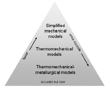
Choosing the correct welding simulation method in Abaqus is not a one-size-fits-all decision; it requires alignment with the primary engineering objective, available computational resources, and required fidelity. The three primary methodologies form a hierarchy of complexity and accuracy.
2. Method 1: Sequentially Coupled Thermomechanical Analysis
The industry-standard approach for high-fidelity prediction of residual stress and detailed distortion.
2.1. Core Workflow
- Step 1 – Transient Thermal: Simulate the heat transfer with a moving source (DFLUX/HETVAL).
- Step 2 – Data Transfer: Export temperature history via
.filor.odbfile. - Step 3 – Static Mechanical: Import temperatures as predefined field and solve with temperature-dependent elastoplastic material.
2.2. When to Use This Method
- Primary Goal: Accurate residual stress prediction for fatigue assessment.
- Required Output: Complete 3D stress tensor, detailed distortion modes.
- Typical Applications: Critical aerospace welds, nuclear component assessment, validation studies.
- Computational Cost: High (hours to days for moderate models).
2.3. Key Implementation Strategy
*IMPORT, STATE=NO, UPDATE=NO
*IMPORT, FILE=ThermalJob, STEP=1
Enable geometric nonlinearity (NLGEOM) and use temperature-dependent kinematic hardening to capture the Bauschinger effect during thermal cycling.
3. Method 2: Fully Coupled Temperature-Displacement Analysis
A simultaneous solution of thermal and mechanical fields within a single analysis step.
3.1. Core Workflow
- Single analysis using coupled temperature-displacement elements (C3D8T, C3D20T).
- Moving heat source applied via user subroutine.
- Material model includes thermal expansion and temperature-dependent plasticity in real-time.
3.2. When to Use This Method
- Primary Goal: Understanding strongly coupled phenomena (e.g., contact resistance changes with pressure).
- Required Output: Interaction between thermal field and stress-induced deformation.
- Typical Applications: Resistance spot welding, friction stir welding (simplified), processes with significant contact pressure changes.
- Computational Cost: Very High (often 3-5× sequential method).
3.3. Key Implementation Strategy
Use explicit dynamics (Abaqus/Explicit) for severe nonlinearities or quasi-static coupled analysis in Standard with small time increments. Convergence is the primary challenge.
4. Method 3: Inherent Strain / Equivalent Load Method
An efficient linear elastic approach for predicting distortion in large structures.
4.1. Core Workflow
- Calibration: Run a detailed local model (Method 1) to extract characteristic plastic strain patterns.
- Application: Map these “inherent strains” as initial conditions (
*INITIAL CONDITIONS, TYPE=SOLUTION) onto a global elastic-only model. - Solution: Single elastic step predicts global distortion.
4.2. When to Use This Method
- Primary Goal: Predicting assembly-level distortion for manufacturing compensation.
- Required Output: Global displacement field, weld sequence optimization.
- Typical Applications: Shipbuilding, large steel structures, automotive frames.
- Computational Cost: Low (minutes to hours after calibration).
4.3. Key Implementation Strategy
The accuracy depends entirely on the calibration model’s representativeness. Use submodeling to extract strains from a detailed local model of a representative joint.
5. Comparative Analysis: Capabilities and Limitations
Table 1: Method Selection Matrix
| Criterion | Sequentially Coupled | Fully Coupled | Inherent Strain |
|---|---|---|---|
| Residual Stress Accuracy | High (when validated) | Highest (theoretically) | Not predicted |
| Distortion Prediction | High fidelity | High fidelity | Good for global shape |
| Computational Time | Medium-High | Very High | Very Low (after calibration) |
| Phase Transformation | Can be included via USDFLD | Can be included | Not applicable |
| Best For | Component-level validation | Process mechanism studies | Large assembly optimization |
| Validation Requirement | Critical (stress & distortion) | Critical (stress & distortion) | Distortion only |
6. Advanced Hybrid and Specialized Methods
6.1. Submodeling for Local Detail
Combine Method 3 (global) with Method 1 (local):
- Run inherent strain analysis on full assembly.
- Cut boundary conditions from global model.
- Apply to detailed local model for stress analysis.
This provides stress focus where needed without full-model computation.
6.2. Computational Weld Mechanics (CWM) for Multi-Pass Welds
For thick-section multi-pass welding:
- Use
*MODEL CHANGE, ADDto activate weld filler elements sequentially. - Implement annealing via
*ANNEAL TEMPERATUREto reset hardening above austenitization temperature. - Employ element birth techniques with “quiet” or “inactive” elements.
6.3. Adaptive Meshing for Severe Deformation
While Abaqus/Standard has limitations, for processes like friction stir welding:
- Use Coupled Eulerian-Lagrangian (CEL) in Abaqus/Explicit for severe material flow.
- Alternative: Arbitrary Lagrangian-Eulerian (ALE) remeshing in third-party preprocessors with Abaqus solver.
7. Critical Implementation Factors Across All Methods
7.1. Material Modeling Consistency
Regardless of method, temperature-dependent properties must cover the full range:
- Solidus to liquidus transition: Implement sharp but continuous property reduction.
- Phase transformations: For steels, account for volumetric change (austenite→martensite: ~4% expansion).
- High-temperature creep: Include time-dependent plasticity (
*CREEP) for slow cooling cycles.
7.2. Heat Source Calibration Protocol
All thermal methods require calibration:
- Match simulated fusion zone to macrograph (adjust a, b, c in Goldak model).
- Match thermal cycles at HAZ locations (adjust efficiency η and convection coefficients).
- Never use literature values without verification for your specific setup.
7.3. Fixture Modeling Philosophy
- Sequential/Full Coupled: Model actual clamps as contact pairs with friction.
- Inherent Strain: Either omit fixtures or include them as elastic constraints if they remain during welding.
- Critical rule: Never over-constrain; use minimum necessary restraint to prevent rigid body motion.
8. Validation Framework: Establishing Credibility
8.1. Tiered Validation Approach
- Level 1 – Thermal: Compare thermo-couple data at 3+ HAZ locations (max ±10% error in peak T).
- Level 2 – Geometric: Match fusion zone dimensions and HAZ width from cross-section (±15%).
- Level 3 – Mechanical: Compare distortion (CMM data) and residual stress (hole-drilling, XRD).
8.2. Acceptable Error Margins for Industry
- Distortion (angular, longitudinal): ±20% of maximum displacement acceptable for design.
- Residual Stress Magnitude: ±30% in heat-affected zone, correct sign (tension/compression) is critical.
- Computational Time vs. Accuracy: Document the trade-off; a method taking 4 weeks that is 5% more accurate than a 1-day method is often not justifiable.
9. Conclusion: Building an Organizational Simulation Strategy
A comprehensive welding simulation capability in Abaqus is not about mastering a single method, but about strategically deploying the right technique for each engineering challenge. For most organizations, we recommend establishing a three-tiered approach:
- Tier 1 (Routine): Inherent strain method for all assembly-level distortion prediction and weld sequence optimization.
- Tier 2 (Detailed): Sequentially coupled analysis for critical joints requiring stress assessment or detailed process development.
- Tier 3 (Research): Fully coupled or specialized methods (CEL, ALE) for fundamental process understanding or novel joining technologies.
The future direction involves integrating these simulations into digital thread workflows—where predicted distortions automatically inform robotic weld paths for compensation, and residual stresses feed directly into in-service fatigue life calculations without manual transfer. The most sophisticated implementation uses machine learning to create surrogate models from detailed simulations, enabling real-time predictions for manufacturing decision support.

