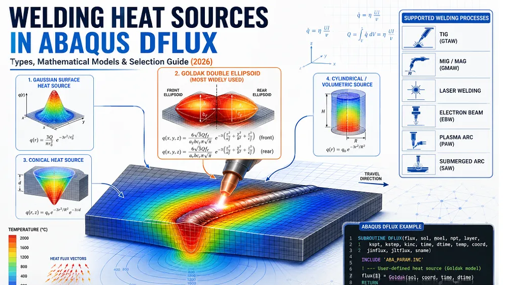
Selecting the right heat source model is one of the most important steps in welding simulation with the Abaqus DFLUX subroutine. Each welding process requires a different mathematical model to represent heat input accurately.
For example, laser welding often uses a Gaussian surface heat source, while arc welding commonly uses the Goldak double-ellipsoid model. Deep-penetration welding usually requires volumetric heat source models.
This article compares the most common DFLUX heat source models, explains their governing equations and key parameters, and helps you choose the best model based on the welding process, penetration depth, and your simulation objectives.
At Mathech, we have guided hundreds of engineers through the complexities of welding simulation. We are here to demystify the Abaqus DFLUX subroutine and provide you with a data-backed roadmap for selecting the right mathematical model for your specific welding process.
What Is a Welding Heat Source? Types and Role in Welding Simulation
In the context of finite element analysis (FEA), a welding heat source is a mathematical representation of the thermal energy input to a workpiece. This heat source is a boundary condition applied to nodes or elements to simulate the heat generated by the arc.
The heat source drives the entire physics of the simulation and determines the thermal cycle, including the peak temperature, heating rate, and cooling rate at every point in the material.
Specifically, the heat source in a welding simulation is quantified by the following parameters:
- Power Input (Q) The total energy delivered to the workpiece surface, measured in Watts (W).
- Efficiency (η) A value below 1.0 that accounts for energy losses caused by radiation, convection, and interaction with the surrounding environment.
- Spatial Distribution Defines how the heat input is distributed across the surface or volume of the material. Different welding processes require different heat source models, such as Gaussian, Goldak double ellipsoidal, or uniform heat distributions.
Types of Welding Heat Sources Used in Abaqus DFLUX
When we discuss Abaqus DFLUX, we are discussing the user subroutine that allows us to define non-uniform, moving heat flux distributions.
| Heat Source Type | Heat Distribution | Typical Welding Applications | Advantages | Limitations |
|---|---|---|---|---|
| Gaussian Surface Heat Source |
Surface heat flux with maximum intensity at the center and exponential decay with radial distance.
Model: q(r) = q0e-3r²/r0² |
|
|
|
| Goldak Double Ellipsoidal Heat Source | A three-dimensional moving heat source consisting of front and rear ellipsoidal regions with different heat distributions. |
|
|
|
| Conical Heat Source | A cone-shaped volumetric heat distribution designed to represent deep penetration welding processes. |
|
|
|
| Uniform Volumetric Heat Source | Constant heat generation inside a defined volume without spatial variation. |
|
|
|
Surface Heat Sources vs Volumetric Heat Sources
The main difference between surface and volumetric heat sources is how the heat input is distributed through the weld region. The appropriate formulation depends on the welding process, penetration depth, and geometry.
Surface Heat Sources: Heat is applied primarily at the material surface using a surface-based flux in Abaqus DFLUX. This approach is suitable when the weld penetration is shallow compared with the material thickness.
For example, a surface Gaussian heat source can be appropriate for shallow penetration welding. However, the actual heat-source model should be calibrated against experimental weld-pool dimensions or measured thermal data whenever possible.
Volumetric Heat Sources: Heat is distributed within a finite volume of the material. In Abaqus, a body heat flux can be implemented through the DFLUX subroutine. This approach is useful for welding processes with significant penetration, where the heat input cannot be represented accurately by a surface flux alone.
Volumetric formulations are commonly used for processes such as GMAW (MIG/MAG), laser welding, and electron beam welding when the process produces substantial penetration. Models such as the double-ellipsoid, conical, and other distributed heat sources can represent the three-dimensional heat-input profile more realistically.
Moving Heat Sources in Welding Simulation
A moving heat source changes its position with time as it travels along the weld path. In an Abaqus DFLUX implementation, the subroutine evaluates the heat flux at the current integration point based on its distance from the instantaneous heat-source location.
Example of source movement
If the heat source moves along the X-axis with a constant welding speed, its center can be described as:
The DFLUX subroutine then calculates the distance between the moving source center and the current integration point (x, y, z). The resulting distance is used to determine the local heat flux according to the selected heat-source equation.
For complex weld paths, the same principle can be extended to curved, multi-pass, or three-dimensional trajectories. Accurate source positioning is critical because an incorrect travel speed, coordinate system, or source location can shift the predicted fusion zone and thermal history.
Distributed Heat Sources for Thick and Thin Plates
The choice of a distributed heat source should consider the penetration depth, weld geometry, material thickness, and welding process. Thickness alone does not determine whether a surface or volumetric model is appropriate.
| Plate Condition | Typical Heat-Source Approach | Modeling Consideration |
|---|---|---|
| Thin Plates | Surface Gaussian or shallow distributed source | Suitable when penetration is shallow relative to the plate thickness |
| Thick Plates | Volumetric sources such as double-ellipsoid or conical models | Captures three-dimensional heat penetration and weld-pool geometry |
| Deep-Penetration Welding | Volumetric or keyhole-oriented heat-source model | Source depth and energy distribution must be calibrated to the weld profile |
Practical recommendation: Do not select a heat-source model only because the plate is thinner or thicker than a fixed value such as 5 mm. Instead, compare the predicted fusion-zone width, penetration depth, and thermal history with experimental or published welding data. This calibration provides a more reliable basis for selecting a Gaussian, double-ellipsoid, conical, or other volumetric heat-source model in Abaqus.
Learn More in Abaqus Welding Simulation
Explore more practical guides on heat sources, Arc Welding, DFLUX Fortran Subroutine, residual stress, Temperature distribution, and Abaqus simulation techniques.
Mathematical Heat Source Models for Welding Simulation
Gaussian Heat Source Model: Theory, Equation, and Applications
The Gaussian distribution is the foundational model for welding. It assumes the heat flux is distributed in a circular pattern on the surface.
Equation:
(Where is the effective radius of the heat source, and ( r ) is the radial distance from the center).

Applications:
- GTAW (TIG) welding.
- Low-current GMAW on thin sections.
- Laser welding (albeit with modifications to account for the keyhole).
- Heat Source Modeling Example: 📂 Abaqus CAE File
- Ready to Use a Complex Abaqus Welding Model?
- Get the complete Abaqus CAE file for welding simulation in spiral path and save hours of modeling time. The file includes the finished geometry, material properties, contact definitions, mesh setup, boundary conditions, loading steps, and analysis configuration. 🛒 Get the CAE File
- Welding Simulation Along a Spiral Path Using DFLUX in Abaqus Metal additive manufacturing (AM)
Pros: Simple to code, computationally cheap.
Cons: Does not account for the “trailing” effect of the weld pool where heat accumulates, leading to an overestimation of the peak temperature at the front and underestimation of the dwell time at the rear.
Goldak Double Ellipsoidal Heat Source Model Explained
Developed by Goldak, Akhlaghi, and others, this model is the industry standard for arc welding.
The double ellipsoid accounts for the asymmetry of the weld pool; the front half is steeper (to represent the arc pushing into the material) while the rear half is wider (representing the heat flowing back into the material).
Equation Structure (Front Half):
Equation Structure (Rear Half):
Where ( ) and ( ) are the fractions of heat in the front and rear, summing to 2.

Applications:
- GMAW (MIG/MAG) welding.
- Submerged Arc Welding (SAW).
- Heavy-section arc welding.
Conical Heat Source Model for Deep Penetration Welding
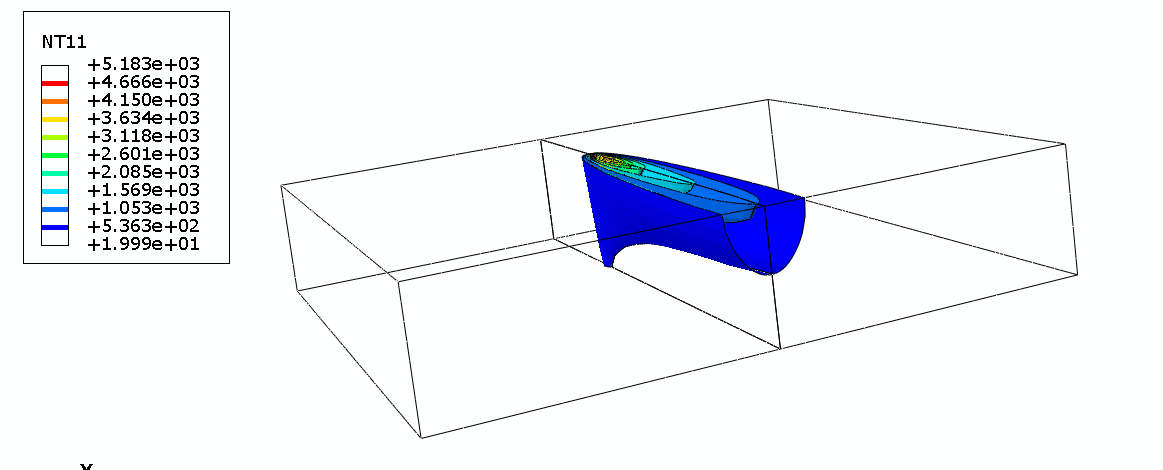
For high-energy density processes like laser welding, the keyhole shape is closer to a cone. The conical heat source applies volumetric heat that decreases linearly with depth.
Equation:
(Where ( r_0(z) ) is the radius at a given depth ( z ), decreasing from the top radius to the bottom radius).
Applications:
- Laser welding.
- Electron Beam Welding.
- Hybrid welding (Laser + Arc).
Which Heat Source Model Is Best for Each Welding Process?
Selecting the right welding heat source model requires engineering judgment. The welding process, heat input, penetration depth, weld-pool geometry, and available experimental data all influence the choice. The following Mathech Engineering Recommendation Matrix for 2026 provides a practical starting point for selecting heat-source models in Abaqus DFLUX welding simulations.
Best Heat Source Models for Arc Welding
| Welding Process | Recommended Heat Source | Engineering Consideration |
|---|---|---|
| GTAW (TIG) | Surface Gaussian | Suitable for shallow penetration. A volumetric Gaussian source may be more appropriate when deeper penetration or multi-pass welding must be represented. |
| GMAW (MIG/MAG) | Goldak Double Ellipsoid | A volumetric model can represent the three-dimensional heat distribution and asymmetric heating around the moving arc. |
| SMAW (Stick) | Goldak Double Ellipsoid | Useful for representing distributed volumetric heat input. The ellipsoid dimensions should be calibrated against the weld-bead geometry. |
| SAW (Submerged Arc Welding) | Goldak Double Ellipsoid | Suitable for high heat input and deep welds. The front and rear dimensions should be adjusted to reproduce the measured thermal profile and weld geometry. |
DFLUX calibration tip: For Goldak-based welding simulations, do not select the a, b, and c parameters arbitrarily. Calibrate the ellipsoid dimensions against the measured weld width, penetration depth, and bead shape whenever reliable experimental data are available.
Best Heat Source Models for Laser Welding
Laser welding requires a different approach because the energy density and penetration profile can vary significantly between conduction and keyhole modes.
| Laser Welding Mode | Recommended Heat Source | Modeling Approach |
|---|---|---|
| Keyhole Mode | Conical or calibrated volumetric source | Represents deep penetration by distributing heat through the weld depth. |
| Conduction Mode | Surface or Volumetric Gaussian | A surface Gaussian can be sufficient for shallow penetration, while a volumetric Gaussian is useful when finite penetration must be represented. |
Abaqus DFLUX tip: For deep-penetration laser welding, the heat-source distribution should reproduce the actual penetration profile. A conical volumetric model is often a practical choice, but its geometry and energy distribution should be validated against the experimental weld cross-section.
Heat Source Models for Electron Beam, Friction Stir, and Hybrid Welding
| Welding Process | Recommended Model | Key Modeling Consideration |
|---|---|---|
| Electron Beam Welding (EBW) | Conical or specialized volumetric source | The high-aspect-ratio penetration profile may require a steep volumetric distribution or a specialized source formulation. |
| Friction Stir Welding (FSW) | Surface + volumetric heat generation | Heat is generated mainly by friction and plastic deformation. Separate contributions from the shoulder and pin can be modeled when required. |
| Hybrid Laser-Arc Welding | Conical + Double Ellipsoid | Combine separate laser and arc heat-source distributions and position them according to the actual process configuration. |
Mathech Engineering Recommendation
Treat the recommendations above as starting points rather than universal rules. The most reliable Abaqus welding heat source model is the one that reproduces the experimentally observed heat distribution, fusion-zone dimensions, penetration depth, and thermal history. When possible, calibrate the DFLUX parameters using measured weld cross-sections and temperature data before using the model for residual stress or distortion prediction.
Some Abaqus Laser Welding Simulation Guides
Explore more practical guides on heat sources, laser welding, residual stress, welding distortion, and Abaqus simulation techniques.
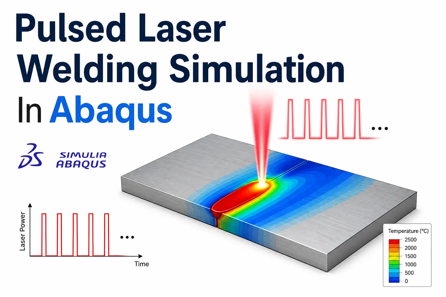
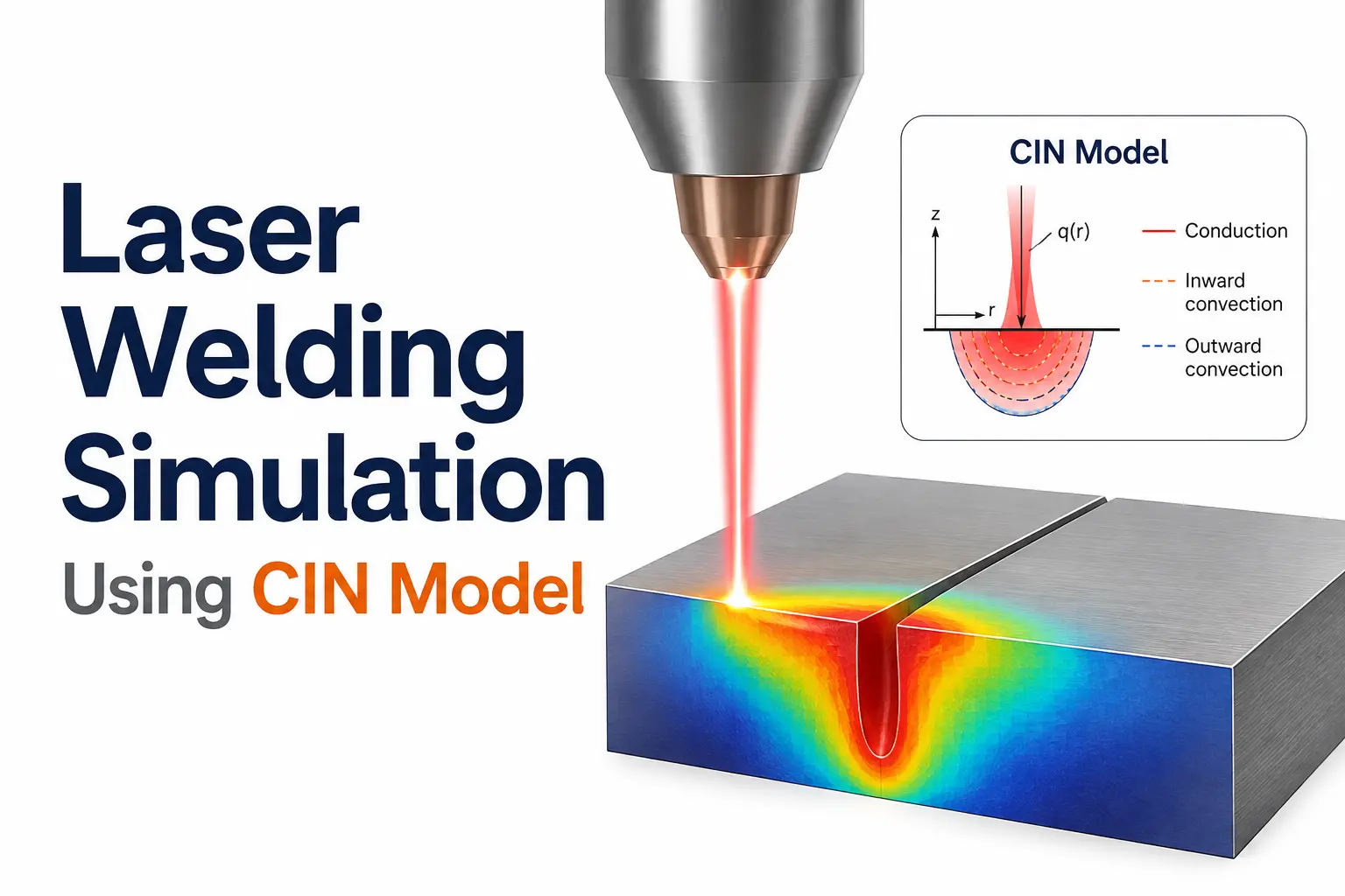
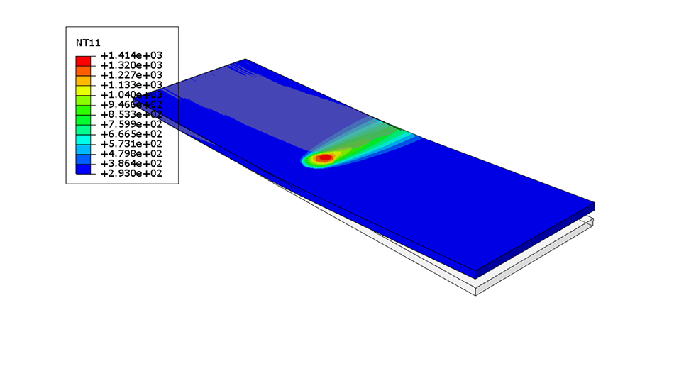
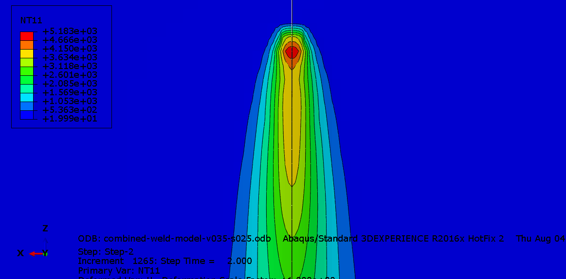
Looking for more welding simulation resources? Browse these Abaqus guides to improve heat-source modeling, thermal analysis, residual-stress prediction, and welding simulation workflows.
| Welding process | Recommended model | Type |
|---|---|---|
| GTAW / TIG | Surface Gaussian | Surface |
| GMAW / MIG | Goldak double ellipsoid | Volumetric |
| SMAW / Stick | Goldak double ellipsoid | Volumetric |
| SAW · Submerged Arc | Goldak double ellipsoid | Volumetric |
| Laser · keyhole | Conical | Volumetric |
| Laser · conduction | Volumetric Gaussian | Volumetric |
| EBW · Electron Beam | Conical | Volumetric |
| FSW · Friction Stir | Surface + volumetric | Surface + vol. |
| Hybrid (Laser + Arc) | Conical + Goldak | Volumetric |
Why Accurate Heat Source Modeling Is Critical in Abaqus Finite Element Analysis
In Abaqus finite element analysis, the accuracy of a welding simulation depends strongly on how the heat source represents the real welding process. A simple uniform heat flux may reproduce the total energy input while still producing an incorrect temperature field, thermal gradient, and cooling rate.
Why Heat Source Accuracy Matters in Welding Simulation
The heat source controls where thermal energy enters the model and how quickly the surrounding material heats and cools. Therefore, its size, shape, intensity, and movement directly affect the thermal history predicted by Abaqus.
An unrealistic heat source can produce reasonable total heat input but incorrect local temperatures. This error propagates into residual stress, welding distortion, phase transformation, and HAZ prediction.
| Welding Simulation Output | Heat Source Influence | Risk of Incorrect Heat Source |
|---|---|---|
| Temperature Distribution | Defines peak temperature, thermal gradients, and heat penetration | Incorrect fusion-zone geometry or heat-affected zone (HAZ) width |
| Residual Stress | Controls thermal expansion, contraction, and the resulting stress field | Incorrect magnitude or distribution of residual stress |
| Welding Distortion | Determines localized heating, thermal shrinkage, and deformation | Incorrect weld deformation, displacement, or buckling behavior |
| Cooling Rate and Microstructure | Controls peak temperature and cooling history around the weld | Inaccurate cooling behavior and phase-transformation prediction |
Heat Source Accuracy and Residual Stress Prediction
Welding creates repeated heating and cooling cycles. The material expands when heated and contracts as it cools. Mechanical restraint prevents this movement from occurring freely, generating plastic deformation and residual stress.
A heat source that is too broad spreads the energy over a larger region. This can produce a smoother temperature field and reduce the local thermal gradients. The resulting Abaqus model may then underestimate the localized thermal-mechanical response.
Relationship Between Heat Input, Temperature Distribution, and Residual Stress
For arc welding, the net heat input per unit weld length can be expressed as:
Here, η is the thermal efficiency, V is voltage, I is welding current, and v is welding speed. The same total heat input can produce very different results when its spatial distribution changes.
| Heat Source Characteristic | Thermal Effect | Welding Simulation Impact |
|---|---|---|
| Highly localized | Steep thermal gradients | Strong localized thermal-mechanical response |
| Broad distribution | Smoother temperature gradients | Potentially incorrect HAZ and stress distribution |
| Incorrect penetration depth | Incorrect through-thickness heating | Incorrect fusion-zone geometry |
Heat Source Calibration for Reliable Abaqus Results
Heat source parameters should not be selected only from theoretical assumptions. A robust Abaqus welding simulation should compare numerical results with experimental measurements.
Typical calibration targets include the fusion-zone dimensions, peak temperature, HAZ width, thermal cycle, and cooling rate. After thermal calibration, the same model can support more reliable residual-stress and distortion predictions.
| Calibration Target | What to Compare |
|---|---|
| Fusion Zone | Width, depth, and overall geometry |
| HAZ | Predicted and measured affected region |
| Thermal Cycle | Peak temperature and cooling history |
| Distortion | Numerical deformation versus experimental measurements |
In welding FEA, the heat source is more than a method for applying energy. It defines the thermal history that drives the mechanical response. Therefore, accurate heat-source geometry, power distribution, travel speed, and calibration are essential for reliable predictions of temperature, residual stress, welding distortion, and HAZ behavior.
Implementing Welding Heat Sources Using the Abaqus DFLUX Subroutine
How the DFLUX Subroutine Defines a Moving Heat Source
The DFLUX subroutine is called for each integration point during the analysis. You must pass the time and the coordinates to the Fortran subroutine.
Logic Flow:
- Calculate the current position of the heat source center:
- Calculate the distance vector from the source center to the integration point:
- Calculate the heat flux intensity using the chosen mathematical model (e.g., Goldak).
- Return the flux value to Abaqus.
Required Parameters for DFLUX Heat Source Modeling
To implement this, you need to define:
- Arc Power (Q): Watts.
- Efficiency (η): Usually 0.75-0.95 for arc welding, 0.8-0.9 for laser.
- Parameters: For Goldak (a, b, c_f, c_r). For Gaussian (r_b). For Conical (r_top, r_bottom, depth).
- Travel Speed (v): mm/sec.
- Start Time: When the arc turns on (usually 0).
- Dwell Time: Time for the heat source to remain at the start (pre-heating) or end (post-heating).
Common Mistakes When Programming DFLUX for Welding Simulation
Even with the right model, engineers often crash the analysis due to programming errors.
- Unit Inconsistency: Ensure your heat flux is in W/mm³ (if using mm units). Check your input parameters. If Q is in Watts and the volume is in mm³, it works. If you are using meters, it’s W/m³.
- Circular Reference: The subroutine must be robust if the integration point is exactly at ( r = 0 ) to avoid division by zero.
- Moving Mesh: If you are using ALE adaptive meshing, the coordinates of the integration points change. Your DFLUX must reference the physical coordinates, not the mesh coordinates.
- Ignoring “Jump” Conditions: Ensure the heat source does not jump if the time step is too large; use DFLUX with a stable time increment.
Best Practices for Selecting a Welding Heat Source Model
Choosing the Right Heat Source Based on Welding Process
The selection process is a trade-off between accuracy and complexity.
- Start with the Process: Determine if the energy transfer is conductive or convective.
- Check the Penetration: If the weld depth is > 2x the width, use a volumetric source (Goldak or Conical).
- Check the Speed: Slow welding creates large, tear-drop pools (Goldak is best). Fast welding creates narrow, conical pools (Conical is best).
Matching Heat Source Parameters with Experimental Data
This is the “calibration” stage. We recommend performing a thermal calibration using thermocouple data from a test weld.
- Method: Run the simulation and compare the thermal cycles at specific points. Iterate the parameters (like “a” and “b” in Goldak) until the simulated temperature history matches the experimental data within +/- 10%.
- Weld Pool Geometry: If you don’t have thermocouples, you can calibrate based on the weld pool cross-section (macrograph). Adjust the power and parameters until the predicted FZ matches the actual weld bead.
Improving Simulation Accuracy While Reducing Computational Cost
A finer mesh is useless if the time step is not optimized.
- Mesh Coarsening: Use a fine mesh near the weld zone (where the heat source is active) and a coarse mesh far away. Use a “clustered” bias toward the weld line.
- Remeshing: If using DFLUX, ensure your element size is smaller than the heat source radius (at least 3-4 elements across the radius). Too coarse a mesh will “average” the flux and reduce peak temperature.
- Time Step: Use an automatically time-incrementing step. Force Abaqus/Standard to take small steps as the heat source passes a node.
Frequently Asked Questions About Welding Heat Sources in Abaqus
Which Heat Source Model Is Most Accurate for Welding Simulation?
A: For arc welding, the Goldak Double Ellipsoid is considered the “gold standard” due to its ability to represent the physical asymmetry of the weld pool. However, “accuracy” is tied to calibration. A simple Gaussian model can be as accurate as Goldak if you calibrate the power and radius carefully for a specific set of experimental data. For laser welding, the Conical model is more accurate.
Can the Goldak Model Simulate Laser Welding?
A: Yes, but with significant modifications. The standard Goldak parameters (specifically “a” and “b”) are designed for large arc welds. To simulate laser welding, you must set the width parameter (“b”) very small (e.g., 0.5 mm) and the depth parameter (“a”) large. However, because the laser produces a “keyhole” effect (where the beam penetrates by vaporizing material), the Conical model is usually a better starting point.
Do All Welding Simulations Require the DFLUX Subroutine?
A: No. If you are performing a simple analysis where the heat source is stationary (e.g., spot welding), you can define a heat flux directly in the interaction module or as a surface heat flux without a subroutine. However, for any moving heat source (GMAW, SAW, Laser welding), you must use the DFLUX user subroutine to define the position, movement, and distribution of the heat over time.
Conclusion: Selecting the Right Welding Heat Source for Reliable Abaqus Simulations
Key Takeaways for Engineers
Selecting a welding heat source is not a “guess.” It is a systematic decision based on:
- Penetration Depth: Surface vs. Volumetric.
- Process Physics: Goldak for arcs; Conical for lasers.
- Calibration: Validation with experiments.
Remember, the best model in the world will fail if your material properties (thermal conductivity, specific heat, latent heat) are incorrect. Always verify your thermal conductivity and density first.
Download Welding DFLUX Examples and Tutorials from Mathech
Are you tired of re-inventing the wheel? At Mathech, we have compiled a library of proven Abaqus DFLUX subroutines and weld simulation templates.
- Download our “Abaqus Weld Simulation Pack” which includes ready-to-use Fortran code for:
- Gaussian Surface Heat Source
- Goldak Double Ellipsoid (Volumetric)
- Conical Volumetric Source
- Access step-by-step video tutorials on calibrating these models against real-world weld data.
- [Download the Free Weld Simulation Toolkit Here]
Need Help? Contact Mathech for Welding simulation
Engineering challenges are rarely solved by one-size-fits-all solutions. If your simulation still refuses to converge, or you are struggling with multi-pass welding, non-linear transient analysis, or crack propagation,bour Abaqus specialists can help you obtain accurate and reliable results.