Modeling Conduction, Convection and Radiation in ABAQUS: A Copper Block Case Study

In our experience, ABAQUS provides powerful capabilities for modeling all three primary heat transfer mechanisms within a single analysis. In this comprehensive tutorial, we walk through a practical case study of a copper block subjected to combined thermal loads, demonstrating step by step how to set up a model that integrates conduction, convection, and radiation alongside multiple boundary conditions and surface interactions.

Understanding the Heat Transfer Problem

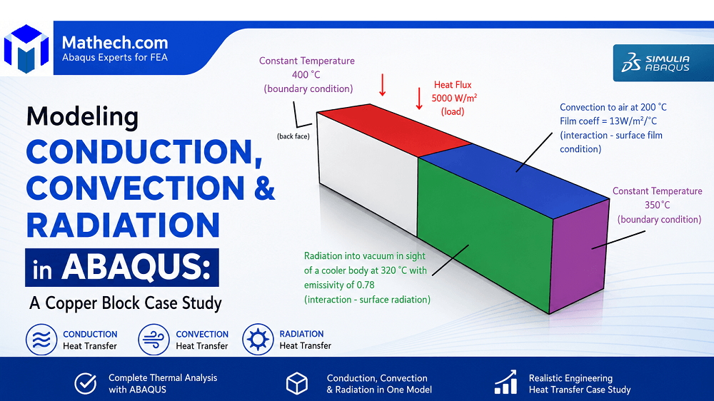
The example we analyze in this tutorial involves a copper block measuring 1m × 1m × 6m subjected to multiple thermal loads. The simulation incorporates:

• Constant temperature boundary condition: 400°C applied to one end face
• Constant temperature boundary condition: 350°C applied to the opposite end face
• Surface heat flux: 5000 W/m² applied to the top face on one portion of the block
• Convection: Heat loss to air at 200°C with a film coefficient of 13 W/m²/°C
• Radiation: Heat loss to a cooler body at 320°C with emissivity of 0.78

The material is copper with thermal conductivity of 401 W/m/°C, which efficiently conducts heat throughout the geometry.

Step 1: Setting Up the Model Environment

Begin by renaming the default model to something descriptive. In the Model Database, right-click on Model-1 and select Rename, changing it to “Heat Transfer.” This organizational step becomes crucial when working with complex models containing multiple analyses.

Step 2: Creating the Part Geometry

The part creation process begins by double-clicking Parts in the Model Database. In the Create Part window:

• Set Name to “Block”
• Keep Modeling Space as 3D
• Set Type to Deformable
• Choose Solid as the Base Feature Shape
• Select Extrusion as the Base Feature Type
• Set Approximate Size to 5

This launches the Sketcher mode where the profile is drawn. Using the Create Lines: Rectangle tool, draw the square profile, then apply dimensions using the Add Dimension tool to set both horizontal and vertical elements to 1m. After completing the sketch, set the extrusion Depth to 6.0 and click OK. The resulting block measures 1m × 1m × 6m.

Step 3: Defining Material Properties

Materials form the backbone of any simulation. To define copper:

1. Double-click Materials in the Model Database
2. Name the material “Copper”
3. Navigate to Thermal → Conductivity
4. Enter a conductivity value of 400 W/mK (approximately 401 W/m/°C, with minor rounding)

This single material property governs how heat propagates through the block in response to various thermal loads.

Step 4: Assigning Sections

Sections link material properties to geometry. The process involves:

1. Double-click Sections in the Model Database
2. Name it “Block Section”
3. Set Category to Solid and Type to Homogeneous
4. In the Edit Section window, select Copper as the material

Next, assign this section to the block by expanding the Parts container, double-clicking Section Assignments, selecting the entire block, and choosing Block Section as the section to apply.

Step 5: Creating the Assembly

Assembly brings the part into the global coordinate system. Double-click Assembly in the Model Database, then expand the Assembly container and double-click Instances. In the Create Instance window:

• Select Block as the part
• Keep Instance Type as Dependent (mesh on part)

This creates an instance of the block in the assembly, ready for meshing and analysis.

Step 6: Partitioning the Block

Partitioning is essential for applying different boundary conditions to different regions of the same part. The block needs to be split into two equal halves:

1. Switch to the Part module using the dropdown at the top of the viewport
2. Click the Create Datum Plane tool, selecting Midway between 2 points
3. Select a corner on one face (0.0,0.0,0.0) and the corresponding corner on the opposite face (0.0,0.0,6.0)
4. Use the Partition Cell: Use Datum Plane tool to create the partition

This partition divides the 6m length into two 3m sections, allowing different thermal loads to be applied to each half.

Step 7: Creating the Analysis Step

Analysis steps define the simulation procedure. For this transient heat transfer problem:

1. Double-click Steps in the Model Database
2. Name the step “Heating Step”
3. Set Insert New Step After to Initial
4. Select Procedure Type: General → Heat transfer
5. In the Edit Step window, set Response to Transient

The transient setting enables time-dependent temperature evolution, essential for understanding how the block heats up and reaches equilibrium.

Step 8: Applying Boundary Conditions

Boundary conditions constrain temperatures at specific locations:

Creating the first temperature boundary condition:

1. Double-click BCs in the Model Database
2. Name it “Const Temp Surf 1”
3. Set Category to Other and Type to Temperature
4. Select the end face on one side of the block
5. Set Distribution to Uniform and specify 400°C

For the second temperature boundary condition:

Follow the same procedure, we select the opposite end face and specifying 350°C. These fixed temperatures establish the primary temperature differential driving heat conduction through the block.

Step 9: Assigning Surface Heat Flux

The heat flux load applies a constant heat input to a specific surface:

1. Double-click Loads in the Model Database
2. Name it “Heat Flux”
3. Set Category to Thermal and Type to Surface heat flux
4. Select the top face of the block on the side closer to the 400°C surface
5. Set Magnitude to 5000 W/m²

This represents heat being applied to one portion of the top surface, simulating a heating element or concentrated heat source.

Step 10: Defining Convection Interaction

Convection models heat transfer from the surface to the surrounding fluid:

1. Double-click Interactions in the Model Database
2. Name it “Convection”
3. Set Types for Selected Step to Surface film condition
4. Select the face where heat will be lost by convection
5. In the Edit Interaction window:

• Set Definition to Embedded Coefficient
• Set Film coefficient to 13 W/m²/°C
• Set Sink temperature to 200°C
• Set Sink amplitude to Ramp

The film coefficient of 13 W/m²/°C represents moderate natural convection in air, while the 200°C sink temperature represents the surrounding air temperature.

Step 11: Configuring Radiation Interaction

Radiation heat transfer becomes significant at elevated temperatures:

1. Create a new interaction named “Radiation”
2. Select Surface radiation as the type
3. Choose the face that will lose heat by radiation
4. In the Edit Interaction window:

• Set Emissivity distribution to Uniform
• Set Emissivity to 0.78
• Set Ambient temperature to 320°C
• Set Ambient temperature amplitude to Ramp

An emissivity of 0.78 is typical for oxidized copper surfaces, and the 320°C ambient temperature represents the surroundings within the line of sight.

Step 12: Generating the Finite Element Mesh

Mesh quality directly impacts solution accuracy:

1. Enter the Mesh module by double-clicking Mesh under the Block part
2. Using Mesh → Element Type, select the entire block
3. In the Element Type window:

• Set Element Library to Standard
• Set Geometric Order to Linear
• Set Family to Heat Transfer
• This selects DC3D8 (8-node linear heat transfer brick elements)

1. Apply global seeding through Mesh → Seed → Part

• Set Approximate global size to 0.5

1. Generate the mesh using Mesh → Part

• Click Yes when prompted to mesh the part

The 0.2 global element size produces a mesh with approximately 750 elements along the length and 5×5 elements in cross-section, providing a reasonable balance between accuracy and computational efficiency.

Step 13: Submitting the Analysis Job

With all definitions complete, the simulation is ready to run:

1. Double-click Jobs in the Model Database
2. Name the job “HeatTransferJob”
3. Set Source to Model and select Heat Transfer
4. In the Edit Job window, set Description to “Job simulates heat conduction through block”
5. Right-click on HeatTransferJob and select Submit

The solver processes the model, and successful completion messages confirm that:

• The input file was processed correctly
• Abaqus/Standard completed successfully
• The job completed successfully

Step 14: Visualizing Results

After the analysis completes:

1. Right-click on HeatTransferJob (Completed) and select Results
2. The Visualization module opens with the ODB file loaded
3. Change to the left view by enabling the Views toolbar and clicking Apply left view

Temperature contours display how heat distributes through the block, revealing hot and cold regions, temperature gradients, and the influence of different boundary conditions. The left view orientation provides the best perspective for understanding the temperature distribution along the length of the block.

Key Learning Points

This tutorial demonstrates several essential ABAQUS concepts:

Multiple thermal mechanisms: The model simultaneously incorporates conduction within the material, convection to surrounding air, and radiation to cooler surroundings. In fact, this combination reflects real-world engineering scenarios where multiple heat transfer pathways act together. For this reason, the analysis provides valuable insights for practical thermal design challenges.

Material property importance: Copper’s high thermal conductivity (401 W/m/°C) ensures rapid heat spread, affecting the overall temperature distribution and the relative influence of surface boundary conditions.

Partitioning strategy: Splitting the block enables different loads to be applied to different regions of the same part, a technique useful for modeling components with varying boundary conditions.

Transient analysis: The transient step setting captures how temperatures evolve over time, essential for processes where thermal response time matters.

Conclusion

This step-by-step tutorial provides a solid foundation for conducting heat transfer analysis in ABAQUS. First, the combination of conduction, convection, and radiation mechanisms in a single model demonstrates the software’s capability to handle complex thermal phenomena. Next, by following these procedures and understanding the underlying principles, we can extend these techniques to analyze heat transfer in diverse applications including electronics cooling, thermal management systems, materials processing, and aerospace components.

Furthermore, the key to successful thermal analysis lies in proper boundary condition application, appropriate material property definition, and quality mesh generation. Finally, with these fundamentals mastered, we can confidently use ABAQUS as a powerful tool for predicting thermal behavior and optimizing designs for thermal performance.