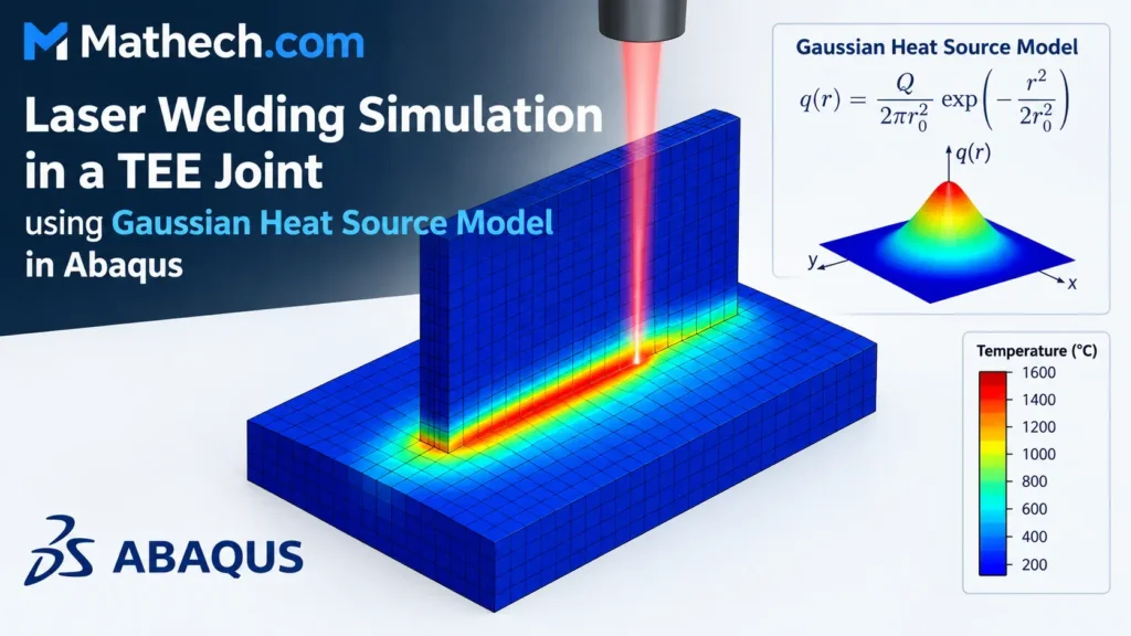
Welding Simulation in TEE joint requires a different modeling strategy from a conventional butt-welded plate. The intersecting plates create a three-dimensional heat-flow path, variable weld geometry, and strong thermal gradients around the joint intersection.

For a laser welding simulation in Abaqus, the most important modeling decisions are the heat-source coordinate system, laser travel path, Gaussian radius, absorbed power, mesh density, and temperature-dependent material properties.

This article presents a practical workflow for implementing a moving Gaussian heat source for a TEE joint and evaluating the resulting temperature field, heat-affected zone, cooling behavior, and thermal history.

Show Table of Contents

1. TEE Joint Geometry for Laser Welding Simulation

A representative TEE joint consists of a base plate and a vertical plate joined along their intersection. For the laser welding simulation in Abaqus, the geometry should provide sufficient space around the weld to capture the thermal gradients and heat-affected region.

The following parameters define a practical example for the Gaussian Heat Source Model:

Parameter	Example Value
Base plate length	100 mm
Base plate width	100 mm
Base plate thickness	5 mm
Vertical plate height	50 mm
Vertical plate thickness	5 mm
Weld length	100 mm
Laser travel direction	Global X
Laser power	1000 W
Absorption efficiency	0.8
Gaussian radius	3 mm
Travel speed	10 mm/s

Important: These values are example parameters, not universal welding conditions. Actual laser power, absorption efficiency, Gaussian radius, and travel speed should be obtained from the experimental process or welding procedure being simulated.

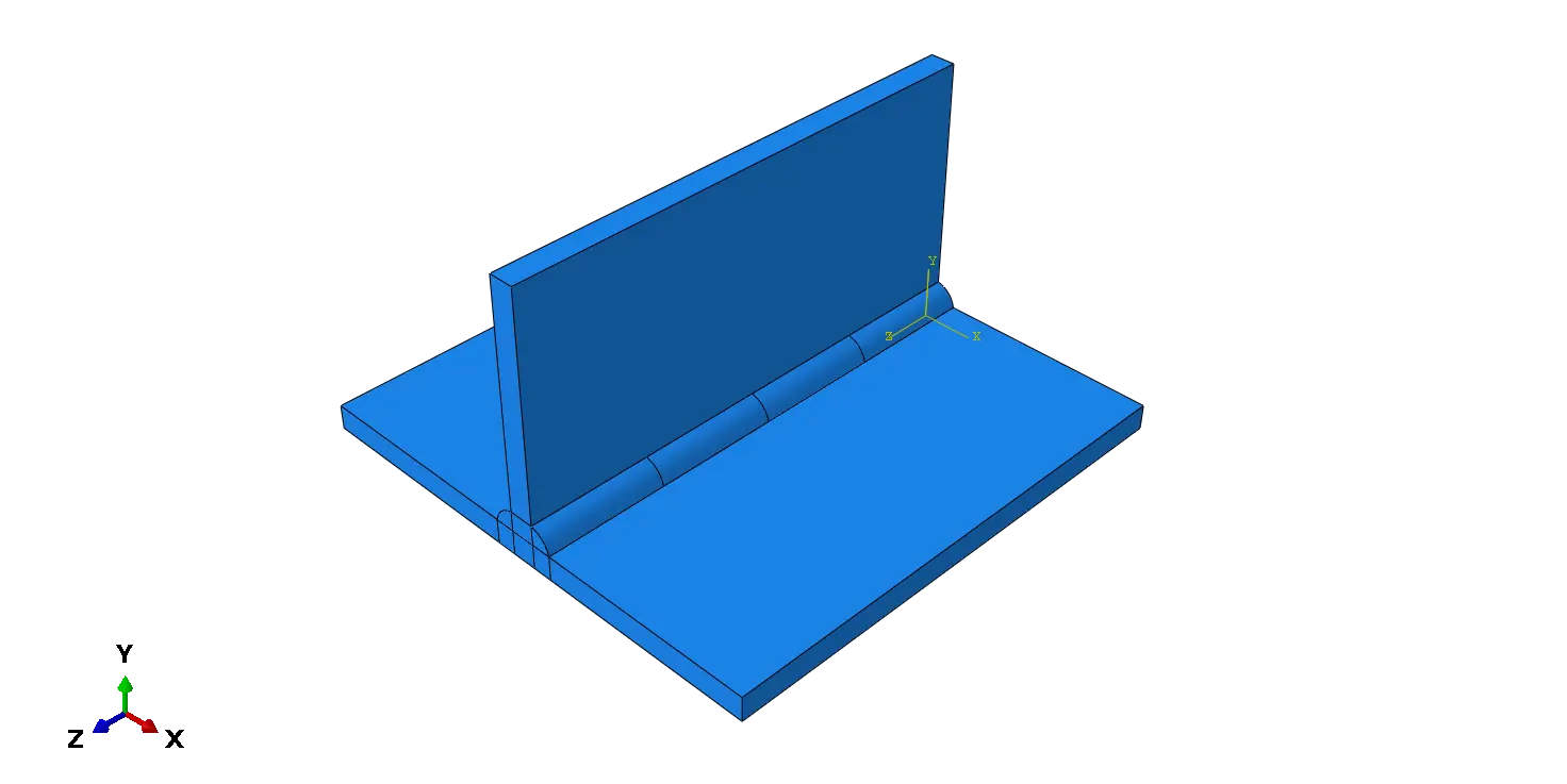
TEE joint GEometry for Laser Welding in Abaqus

TEE joint geometry and assembly used for laser welding simulation in Abaqus.

The vertical plate should intersect the base plate without creating unintended gaps or overlaps. The geometry at the intersection directly affects the local heat-flow path and therefore the predicted temperature distribution.

For a thermal-only model, the two plates can be represented as a single connected thermal domain when the primary objective is temperature prediction. However, separate parts with appropriate interaction definitions may be preferable when the model will later be extended to thermo-mechanical analysis, residual stress, or welding distortion.

Geometry Considerations for the TEE Joint

The TEE intersection deserves particular attention because the local heat-flow direction changes rapidly around the weld. Before generating the Abaqus mesh, verify the following:

The base and vertical plates intersect correctly.
The weld path is geometrically continuous.
No unintended gaps or overlaps exist at the joint.
The laser travel direction is clearly defined.
The heat-source location can be mapped to the weld centerline.
The element size near the weld is sufficiently small to resolve the Gaussian heat distribution.

Modeling note: A geometrically incorrect TEE intersection can produce smooth and visually convincing temperature contours while still giving physically incorrect thermal results. Always verify the weld path and heat-source position before performing a detailed mesh or parameter study.

ABAQUS & ENGINEERING SIMULATION

Need Help With Your Welding Simulation Project?

Get expert support for Abaqus modeling, FEA, thermal analysis, welding simulation, material modeling, and complex engineering problems.

Request a Project Contact an Expert

Tell us about your project, requirements, simulation type, and timeline.

2. Transient Heat Transfer Step in Abaqus

For a laser welding thermal model, a transient heat transfer analysis is normally appropriate. The transient formulation allows the model to capture the moving laser, rapid temperature changes, and subsequent cooling of the TEE joint.

In Abaqus/Standard, create a transient heat transfer step and define the total welding time from the weld length and laser travel speed:

t_weld = L_weld v

where:

L_weld is the welding length.
v is the laser travel speed.

Example: If the laser travels 80 mm at a speed of 5 mm/s, the welding time is:

t_weld = 80 mm 5 mm/s = 16 s

The analysis should normally continue beyond the end of laser travel when the cooling stage is important. This allows the model to capture the thermal cycle after the heat source leaves the joint and provides more useful information about the cooling rate and residual thermal field.

Recommended Abaqus Welding Simulation Sequence

A practical simulation sequence for the TEE joint can be organized into the following stages:

1 Initial temperature definition: Assign the initial temperature of the TEE joint before laser heating begins.
2 Transient laser heating: Activate the moving Gaussian heat source through the DFLUX subroutine.
3 Laser movement along the TEE joint: Move the heat source continuously along the predefined weld centerline.
4 Post-welding cooling: Continue the analysis after laser shutdown to capture the cooling thermal field.
5 Thermal-history extraction: Extract temperature versus time at selected locations around the weld.
6 Experimental comparison: Compare the predicted thermal cycles and weld dimensions with experimental measurements.

3. Moving Gaussian Heat Source for Laser Welding

The Gaussian heat source should move continuously along the weld path during the laser welding simulation. For a surface-based Gaussian distribution, the applied heat flux can be expressed as:

q(r,t) = 2ηP πr₀² exp ( − 2r² r₀² )

where:

P = laser power.
η = absorption efficiency.
r₀ = Gaussian beam radius.
r = distance from the instantaneous laser center.

We use a Fortran subroutine to apply the heat from laser welding using a Gaussian model. Here you can read more about how to link Fortran and Abaqus.

Absorbed Laser Power

The heat source should account for the fraction of laser power absorbed by the material. The absorbed laser power is:

P_abs = ηP

For a laser power of 1000 W and an absorption efficiency of 0.8:

P_abs = 0.8 × 1000 = 800 W

Moving Laser Source Position

The position of the Gaussian heat source changes with time as the laser travels along the weld. If the laser moves in the global X direction, its instantaneous center can be defined as:

x_c(t) = x₀ + vt

where x₀ is the initial laser position and v is the laser travel speed.

For a source moving over a planar surface, the radial distance from the instantaneous laser center can then be calculated as:

r² = (x − x_c)² + (y − y_c)²

Important for TEE Joint Modeling

The planar formulation above is not sufficient for a typical TEE joint. The weld region is not necessarily located on a single global plane, and the local surface orientation changes around the intersection of the two plates. Therefore, the heat-source coordinates should be defined relative to the actual weld path or a suitable local coordinate system.

For the TEE-joint model, the next step is to replace the simple global-coordinate distance calculation with a local weld-coordinate formulation. This allows the Gaussian heat source to remain correctly positioned along the weld centerline throughout the Abaqus simulation.

4. Local Weld Coordinate System for the Gaussian Heat Source in TEE Joint

The most important improvement over a simple plate model is to define the heat source using a local weld coordinate system. This allows the Gaussian distribution to follow the actual weld trajectory instead of relying only on global X-Y coordinates.

Define three local unit vectors:

e_t = tangent vector along the welding direction.
e_n = local surface normal.
e_w = transverse direction across the weld.

Moving Laser Center

The laser center can then be described using the initial weld position, welding speed, and local tangent vector:

x_c(t) = x₀ + vt e_t

At every time increment, the instantaneous laser center is updated along the welding direction. This makes the heat source move continuously along the weld path.

Local Coordinates at Each Integration Point

For each integration point, calculate its position relative to the moving laser center. The resulting vector can then be projected onto the local weld coordinate directions.

The local coordinates perpendicular to the welding direction define the distance from the laser center.

r² = ξ² + ζ²

Here, ξ and ζ are the local coordinates perpendicular to the laser travel direction. They determine how far each integration point is from the instantaneous center of the Gaussian heat source.

Why Use Local Coordinates?

This approach is considerably more robust than defining the Gaussian distribution directly in global X-Y coordinates. The heat source can follow the weld trajectory even when the weld orientation changes relative to the global coordinate system.

Why This Matters for a TEE Joint

A TEE joint introduces a geometric complication because the base plate and vertical plate have different surface orientations. The weld region therefore cannot always be represented accurately using a single global plane.

Follow the Actual Weld Trajectory

If the laser interacts primarily with the fillet region, the heat source should follow the actual weld trajectory, not simply a line defined in the global coordinate system. Otherwise, the heat flux may move too far from the physical weld region as the laser travels.

Practical Abaqus Implementation

Define the weld centerline and its travel direction.
Calculate the local tangent vector e_t.
Define the local transverse and normal directions.
Update the laser center according to the welding speed and simulation time.
Project each integration-point position into the local coordinate system.
Use the local transverse coordinates to evaluate the Gaussian heat flux.

In Abaqus, this local-coordinate formulation provides the foundation for a more reliable DFLUX implementation, especially when modeling laser heating around complex weld geometries such as TEE joints.

Welding Simulation Resources

More Abaqus Laser Welding Simulation Guides

Explore more practical guides on heat sources, laser welding, residual stress, welding distortion, and Abaqus simulation techniques.

Learn how to do Pulsed laser welding simulation in Abaqus

Pulsed Laser Welding Modeling in Abaqus

Learn how to model pulsed laser heat input and thermal behavior.

Laser Welding Simulation in Abaqus Using CIN Heat Source Model

Laser Welding Simulation Using the CIN Model

See how the CIN model can represent deep-penetration laser welding.

How to Simulate and Analyze Laser Welding in Abaqus

Follow a practical workflow for laser welding analysis using Abaqus.

How to do Laser Hybrid Welding Simulation in Abaqus

Laser-Arc Hybrid Welding Simulation in Abaqus

Explore Abaqus modeling strategies for laser-arc hybrid welding.

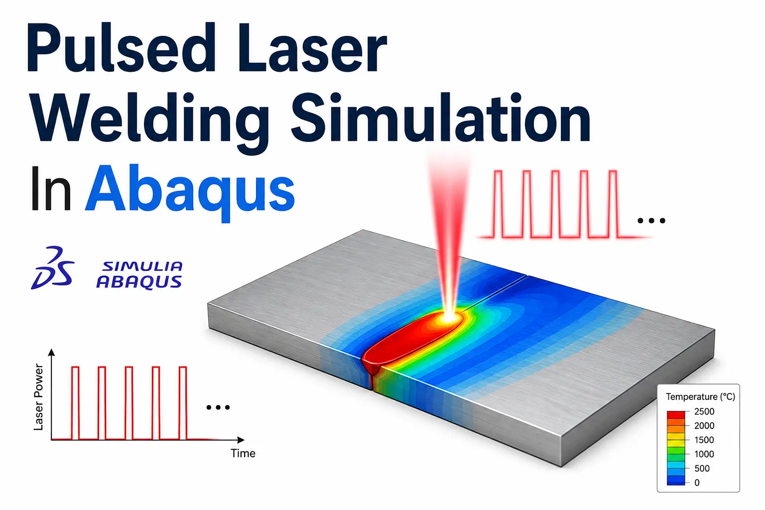
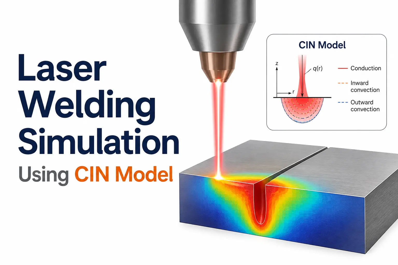
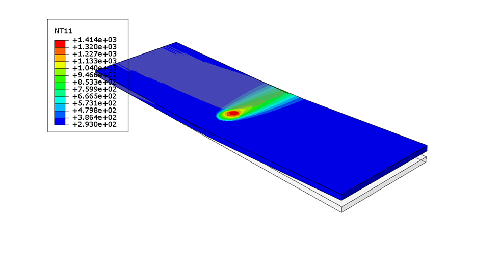
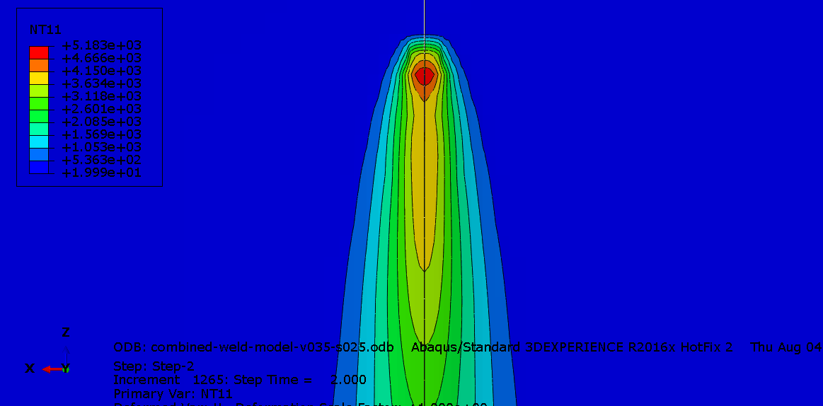
Looking for more welding simulation resources? Browse these Abaqus guides to improve heat-source modeling, thermal analysis, residual-stress prediction, and welding simulation workflows.

5. Implementing the Heat Source with DFLUX

ABAQUS IMPLEMENTATION

A practical laser welding simulation in Abaqus can implement the moving Gaussian heat source using the DFLUX user subroutine. DFLUX allows the applied heat flux to change with the laser position and welding conditions throughout the transient analysis.

Parameters Available to DFLUX

Time
Current analysis time

Position
Current integration-point coordinates

Step
Analysis step number

Increment
Current increment number

Laser Power
Nominal or absorbed power

Welding Speed
Heat-source travel speed

Gaussian Radius
Spatial heat distribution

Travel Direction
Laser movement vector

Local Coordinates
Weld-based heat-source system

DFLUX Heat-Source Logic

01 Read the current integration-point coordinates.

02 Read the current analysis time.

03 Calculate the instantaneous laser-center position.

04 Calculate the distance from the laser center.

05 Evaluate the Gaussian heat-flux distribution.

06 Apply the heat flux within the defined laser interaction region.

07 Return the calculated value through FLUX.

Simplified DFLUX Example- Laser Moving Along X

XC = X0 + V * TIME(2)

R2 = (COORDS(2)-Y0)**2 +
     (COORDS(3)-Z0)**2

FLUX(1) = (2.D0*ETA*POWER) /
     (PI*R0**2) *
     EXP(-2.D0*R2/R0**2)

Temperature contour in laser welding simulation in Abaqus | TEE joint

Temperature distribution contour in TEE Joint Laser Welding Simulation

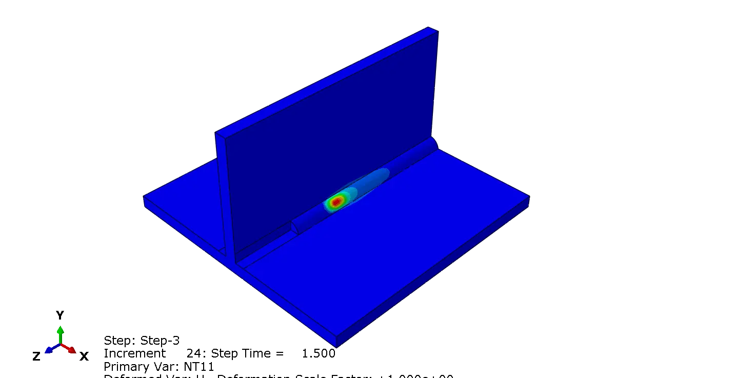
Important for TEE-Joint Welding

The code above is only a simplified representation of a moving Gaussian heat source. It assumes a fixed global plane and a laser moving along the X direction. A realistic TEE-joint Abaqus model should instead use the actual weld trajectory and a local weld coordinate system. This is particularly important because the base plate and vertical plate have different surface orientations.

Practical Implementation Strategy

For a TEE joint, define the weld centerline first. Then calculate the laser center from the welding speed and analysis time. Project the current integration-point position into the local weld coordinate system and evaluate the Gaussian distribution using the local transverse distances. This approach provides a more robust DFLUX implementation and can later be extended to curved welds and complex laser trajectories.

Gaussian Body Heat Flux in Laser Welding Simulation | TEE joint

Applying Body Heat Flux of Laser Welding in TEE joint

6. Defining the Parameters for Laser Welding in a TEE Joint

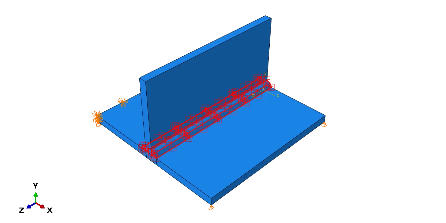
For a TEE joint laser welding simulation in Abaqus, a useful approach is to define the laser centerline along the intersection between the two plates. This allows the moving heat source to follow the actual weld path instead of relying only on fixed global coordinates.

Suppose the weld path is represented by:

x_w(s)

where s is the distance measured along the weld path. The laser center can then be defined as:

x_c(t) = x_w(vt)

This formulation is especially useful when the weld path is curved or when the joint geometry becomes more complicated. The heat source can follow the weld geometry directly, making the model easier to extend and maintain.

STRAIGHT WELD

Straight TEE Joint

For a straight weld path, the laser center can be described using the initial position and the welding direction:

x₀ + vte_t

CURVED WELD

Curved Weld Path

For a curved weld, the laser center should be evaluated directly from the mathematical or geometric representation of the weld path.

A Scalable Laser-Welding Framework

Defining the laser position from the weld trajectory provides a scalable framework for extending an Abaqus welding model to more complex geometries and manufacturing paths.

Curved TEE joints

Circular welds

Pipe-to-plate joints

Nozzle connections

Multi-pass welding

Robotic laser trajectories

6.1. Choosing the Gaussian Radius

The Gaussian radius strongly affects the predicted weld pool, temperature distribution, and thermal gradient. It should therefore be treated as an important calibration parameter rather than an arbitrary input.

Smaller r₀

Higher peak heat flux.
Higher local temperature.
Narrower heated region.
Steeper thermal gradients.

Larger r₀

Lower peak heat flux.
Wider temperature distribution.
Lower local temperature.
Broader thermally affected region.

q_max = 2ηP / (πr₀²)

The peak heat flux varies with 1/r₀². Therefore, changing the Gaussian radius from 2 mm to 1 mm does not simply double the peak heat flux. It increases the peak value by a factor of four.

Calibration tip: Calibrate the Gaussian radius against experimental weld-pool dimensions, penetration depth, and thermal response instead of selecting it arbitrarily.

6.2. Laser Power and Absorption Efficiency

The thermal model should use the absorbed laser power, not automatically the nominal laser power.

P_abs = ηP

Parameter	Value
Laser power	1000 W
Absorption efficiency	0.80
Absorbed power	800 W
Welding speed	5 mm/s
Nominal line energy	200 J/mm
Absorbed line energy	160 J/mm

Laser Line Energy

The nominal linear energy is:

E_l = P / v

The absorbed linear energy is:

E_l,abs = ηP / v

For the example:

E_l = 1000 / 5 = 200 J/mm
E_l,abs = 800 / 5 = 160 J/mm

These values provide a useful first-order check of whether the simulated thermal response is physically reasonable.

7. Temperature-Dependent Material Properties for Laser Welding

Using constant material properties can produce significant errors in a laser welding simulation.

At minimum, define temperature-dependent:

Thermal conductivity.
Specific heat.
Density.

For a more realistic model, account for the melting range and latent heat.

A typical material definition should therefore follow the form:

Property	Temperature dependence
Density	Required
Conductivity	Required
Specific heat	Required
Latent heat	Recommended
Solidus temperature	Required for melting treatment
Liquidus temperature	Required for melting treatment

Thermal conductivity can change substantially with temperature. Specific heat may also increase around phase transformation regions.

If these effects are ignored, the predicted peak temperature and cooling rate may be misleading.

8. Initial and Boundary Conditions of TEE Joint

Set the initial temperature according to the physical welding condition.

For room-temperature welding:

$T_0=T_{\mathrm{amb}}$

A typical value may be:

$T_0=25^\circ C$

Apply heat losses from exposed surfaces using convection and radiation.

The convective heat loss can be represented by:

h(T-T_{\mathrm{amb}})

Radiation can be represented by:

$\epsilon\sigma \left(T^4-T_{\mathrm{amb}}^4\right)$

Both mechanisms can become important during the cooling stage.

For a laser welding simulation, radiation becomes increasingly important at high temperature, so using only a constant convection coefficient may not provide sufficient accuracy.

9. Mesh Strategy for Laser welding of the TEE Joint

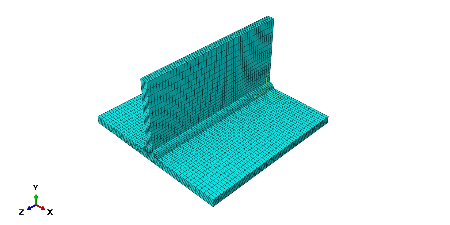
Mesh density has a direct effect on the predicted temperature gradients.

The highest mesh density should be concentrated around:

The laser path.
The weld region.
The TEE intersection.
Expected fusion-zone boundaries.
The heat-affected zone.

A practical strategy is:

Fine mesh

Near the weld and laser path.

Intermediate mesh

Around the heat-affected zone.

Coarse mesh

Far from the weld where temperature gradients become small.

The mesh should not be uniformly fine throughout the entire model unless the geometry is small enough to justify the additional computational cost.

Mesh part in Abaqus for Welding simulation | TEE joint

Recommended element type

For a three-dimensional transient thermal analysis, an 8-node brick heat-transfer element such as DC3D8 is often a practical choice. Check it out here to see how to select right element type for welding models.

Where geometry requires greater flexibility, tetrahedral thermal elements can be used, but the resulting mesh should be checked carefully around the weld.

Mesh Independence Study

A single mesh should not be trusted simply because the temperature contour looks smooth.

Run at least three mesh levels around the weld. See this article to Learn How to mesh a 3D model in Abaqus

For example:

Mesh	Weld-region element size
Coarse	2.0 mm
Medium	1.0 mm
Fine	0.5 mm

Compare:

Maximum temperature.
Peak temperature at selected points.
Fusion-zone dimensions.
HAZ width.
Cooling rate.
Thermal cycle.

If the difference between the medium and fine mesh is small, the medium mesh may provide a better balance between accuracy and computational cost.

This is particularly important for a Gaussian heat source because the heat flux changes rapidly over a small distance.

10. Time Increment Selection

The time increment must resolve the movement of the laser.

The approximate laser movement during one increment is:

$\Delta x=v\Delta t$

A useful practical condition is to ensure that the laser does not move several element lengths during one increment.

For example, if:

$v=5;mm/s$

and the weld-region element size is:

$\Delta x_e=0.5;mm$

then an increment corresponding to approximately 0.1–0.25 mm of laser movement provides much better spatial resolution than allowing the laser to jump several millimeters between increments.

The exact increment should also be controlled by thermal convergence and the characteristic heating time.

11. Temperature Results to Extract

The temperature contour alone is not sufficient to validate the model.

Extract temperature histories at several locations around the TEE joint.

Recommended monitoring points include:

Directly below the laser center.
On the base plate beside the weld.
On the vertical plate beside the weld.
At the expected HAZ boundary.
Several millimeters away from the weld.
At different distances along the welding direction.

For each point, obtain:

T(t)

The thermal cycle can then be evaluated in terms of:

Peak temperature.
Heating rate.
Cooling rate.
Time above critical temperatures.
Thermal gradients.

12. Common Problems in Laser Welding Simulation in Abaqus

TROUBLESHOOTING

Several problems can occur when implementing a Gaussian heat source and DFLUX for laser welding in Abaqus. The following checks help identify whether the problem comes from the heat-source formulation, mesh, material properties, or model setup.

12.1 Heat Source Is Applied to the Wrong Surface

This is one of the most common problems in Abaqus laser welding simulations. A global-coordinate Gaussian source may move correctly along the welding direction but fail to remain centered on the actual fillet region.

Recommended solution Define the heat source using a local weld coordinate system and make the laser center follow the actual weld trajectory.

12.2 Peak Temperature Becomes Unrealistically High

An excessively high peak temperature does not necessarily mean that the laser power is too large. The problem may originate from the spatial distribution of the heat source or the thermal properties of the material.

Gaussian radius

The radius may be too small.

Absorption

Absorption efficiency may be too high.

Mesh

The weld-region mesh may be too coarse.

Surface area

Heat flux may be applied to an incorrect area.

Material data

Thermal properties may be incomplete.

Phase change

Melting or latent-heat effects may be ignored.

Do not immediately reduce laser power First verify the absorbed-energy calculation, Gaussian distribution, heat-source location, mesh resolution, and material properties. Only then adjust the laser power or absorption efficiency.

12.3 Temperature Field Is Too Wide

If the simulated thermal field spreads much farther than the experimental weld region, check both the heat-source distribution and the thermal properties.

Gaussian radius may be too large.
Thermal conductivity may be too low.
Welding speed may be too low.
Heat may be distributed over an excessively large area.

Compare weld dimensions before changing parameters Compare the predicted fusion-zone width and HAZ width with experimental measurements before modifying the heat-source parameters.

12.4 Temperature Contours Are Discontinuous

Discontinuous temperature contours can indicate a problem with the mesh, heat-source position, time resolution, or element connectivity.

Check the following:

Mesh topology.
Laser-source position.
Time resolution.
Element connectivity.
Regions receiving the applied heat flux.

Useful diagnostic Plot or inspect the laser position relative to the mesh before running a long transient simulation. This simple check can reveal an incorrect source trajectory early.

12.5 DFLUX Produces Zero or Negligible Heat Flux

A DFLUX subroutine can return zero or negligible heat flux when the calculated laser position does not intersect the active model region. This is especially important when using a moving Gaussian heat source.

01. Coordinates

Check model units.

02. Start Position

Verify the laser origin.

03. Direction

Check travel direction.

04. Speed

Verify welding speed.

05. Time

Check the DFLUX time variable.

06. Radius

Check Gaussian radius.

07. Activation

Check active surfaces/elements.

08. Coordinates

Verify the local system.

Simple DFLUX Diagnostic

Temporarily inspect the calculated laser-center coordinates during the analysis. Confirm that the laser center starts at the intended weld location and moves along the complete weld path. If the calculated position leaves the active model region, the Gaussian function can become effectively zero.

Recommended Troubleshooting Sequence

When a laser welding simulation produces unexpected temperatures or heat-flux results, troubleshoot the model in a controlled sequence rather than changing several parameters at once.

Verify the laser trajectory and local coordinate system.
Check the absorbed laser power.
Verify the Gaussian radius and heat-source distribution.
Check DFLUX coordinates, time, and travel speed.
Verify the applied surface or active elements.
Check mesh resolution near the weld.
Verify temperature-dependent material properties.
Compare fusion-zone and HAZ dimensions with experimental data.

14. Abaqus Workflow for TEE-Joint Laser Welding Simulation

ABAQUS WORKFLOW

A reliable TEE-joint laser welding simulation should follow a controlled sequence from geometry creation to experimental calibration. The workflow below covers the main steps required to build and verify the transient thermal model in Abaqus.

Geometry

Create the base and vertical plates. Verify the TEE-joint intersection and ensure that the weld region has the intended geometry.

Material

Define temperature-dependent thermal properties, including thermal conductivity and specific heat. Add additional high-temperature data when required.

Assembly

Position the base and vertical plates correctly and establish the welding region and weld trajectory.

Define Steps

Create the transient heat transfer step for laser heating and a separate cooling step when post-welding thermal evolution is important.

Initial Temperature

Apply the initial temperature to the model. Use the measured or experimentally specified initial thermal condition rather than assuming an arbitrary value.

Heat Losses

Define convection and radiation on exposed surfaces. Use appropriate ambient temperature, convection coefficient, and emissivity.

Mesh

Refine the mesh around the TEE intersection, weld region, and laser interaction zone. Use a coarser mesh away from regions with steep thermal gradients.

DFLUX

Implement the moving Gaussian heat source using the Abaqus DFLUX subroutine. Use the local weld coordinate system for complex TEE-joint geometry.

Verification

Before running the full analysis, verify the laser position, absorbed energy, heat-flux magnitude, and boundary conditions.

Run Analysis

Run the transient thermal analysis and monitor convergence, temperature evolution, and heat-source behavior during laser travel.

Post-Processing

Extract temperature contours, thermal histories, peak temperatures, and cooling rates. For thermo-mechanical models, evaluate residual stress and distortion after thermal loading.

Calibration

Compare the predicted fusion-zone and HAZ dimensions with experimental data. Calibrate the heat-source parameters based on measured weld characteristics.

Recommended Modeling Logic

The most important point is to complete the verification stage before calibration. First confirm that the DFLUX implementation, laser trajectory, absorbed power, mesh, and thermal boundary conditions are correct. Then use experimental weld dimensions to calibrate the Gaussian heat-source parameters.

From Geometry to Experimental Validation

A robust TEE-joint laser welding model is not defined by the DFLUX subroutine alone. Reliable results require consistent geometry, temperature-dependent material data, appropriate mesh and time resolution, correct heat losses, a physically consistent Gaussian heat source, and experimental validation.

15. Improving the Gaussian Model for Deep-Penetration Laser Welding

A Gaussian heat source may not reproduce a deep-penetration laser weld accurately.

For example, the Laser Welding Simulation Using CIN Model applies heat throughout a three-dimensional volume. This makes it useful for representing narrow and deep penetration in beam welding.

Problems With a Purely Surface-Applied Source

If the real weld exhibits significant penetration, a purely surface-applied Gaussian distribution can produce:

Incorrect penetration depth.
Excessive surface temperature.
Incorrect subsurface thermal gradients.
Incorrect fusion-zone geometry.

Consider a Volumetric Heat Source

In such cases, consider a volumetric heat source or a combined surface-volumetric formulation. A volumetric source distributes heat through the material depth instead of applying all energy only at the surface.

General Volumetric Source

The volumetric heat input can be represented generally as:

Q₀ = f(x, y, z, t)

Here, f controls the spatial distribution of heat through the weld depth and along the moving laser path.

Goldak-Type Alternative

A Goldak-type double-ellipsoidal heat source can also be considered when directional heat penetration needs to be represented. The two ellipsoidal regions can provide different heat distributions ahead of and behind the moving heat source.

Heat-Source Selection for a TEE Laser Weld

For a TEE laser weld, the appropriate heat-source model should be selected from the observed weld morphology. A surface Gaussian source is a practical starting point for shallow penetration, while a volumetric or combined source is more appropriate when the weld is narrow and deep. The source should also follow the actual three-dimensional weld trajectory rather than being defined only from global coordinates.

16. Final Technical Conclusion

A laser welding simulation in a TEE joint using a Gaussian heat source in Abaqus provides an effective approach for predicting temperature distribution, fusion-zone geometry, and HAZ behavior. For accurate results, define the heat source along the actual weld path and calibrate the model using experimental data. For deep-penetration welding, a volumetric or combined heat-source model may provide better accuracy.

17. Resources for Studying Laser Welding Simulation in Abaqus

STUDY RESOURCES

If you want to develop reliable laser welding simulations in Abaqus, study the heat-source formulation, DFLUX implementation, thermal modeling, mesh and time-step selection, and experimental calibration together. The following resources provide a practical path from the Abaqus fundamentals to advanced laser-welding models.

01 · ABAQUS DOCUMENTATION

DFLUX User Subroutine

Learn how Abaqus defines nonuniform surface and body heat fluxes using DFLUX. This is the foundation for implementing a moving Gaussian or volumetric laser heat source.

02 · RESEARCH PAPER

Laser Welding of T-Joints

Study the influence of laser heat-source inclination on melted-zone geometry, deformation, and stress. The paper is especially relevant to T-joint and TEE-joint welding simulations.

03 · ADVANCED RESEARCH

Hybrid Laser-Arc Heat Sources

A useful advanced example of combining laser and arc heat-source models in Abaqus through DFLUX. It also demonstrates experimental validation of temperature and deformation predictions.

04 · PRACTICAL EXAMPLE

CIN Volumetric Heat Source

A practical Abaqus example using DFLUX and a cylindrical involution normal (CIN) heat source for volumetric laser welding. Useful for studying deep-penetration thermal models.

05 · PRACTICAL COURSE

Laser Welding & DFLUX Examples

Covers moving laser beams, Gaussian energy distributions, surface and volumetric heat fluxes, and different laser paths implemented with DFLUX.

06 · VIDEO TUTORIAL

Abaqus Welding Masterclass

Covers moving heat sources, DFLUX, Gaussian welding models, Goldak double-ellipsoid sources, and residual-stress workflows.

Recommended Study Path

01. Learn transient heat transfer in Abaqus.

02. Understand moving Gaussian heat sources.

03. Implement DFLUX with Fortran.

04. Compare surface and volumetric sources.

05. Calibrate against weld-pool geometry.

06. Extend the model to thermo-mechanical analysis.

For laser welding research: Do not choose a heat-source model only because it is easy to implement. Start from the experimentally observed weld-pool shape, penetration depth, and thermal response. Then select and calibrate the heat-source formulation that can reproduce those characteristics.