Welding simulation examples helps engineers and researchers to find the best topics for study the thermal and mechanical effects of welding. Abaqus FEA can predict temperature distribution, thermal cycles, residual stress, welding distortion, heat-affected zones, and plastic deformation.
A realistic Abaqus welding simulation may include moving heat sources, transient heat transfer, temperature-dependent material properties, convection, radiation, and thermo-mechanical analysis.
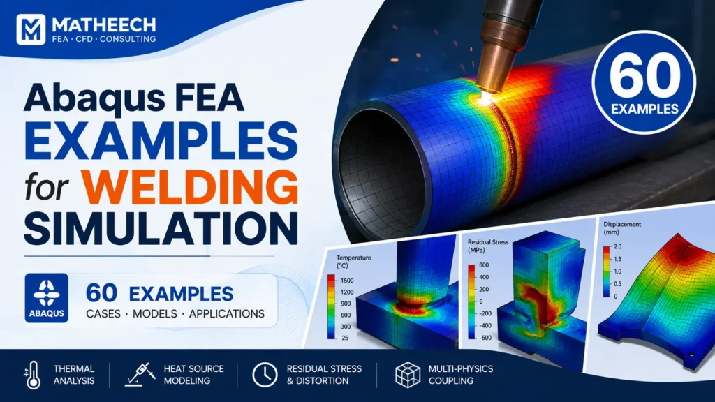
This guide provides 60 Abaqus FEA examples for welding simulation, covering different welding processes, heat sources, geometries, heat-transfer methods, and analysis types. These examples are useful for Abaqus projects, research, thesis work, and engineering consulting.
1. Main Types of Abaqus Welding Simulations
| Classification | Abaqus Welding Simulation Examples |
|---|---|
| Welding Process | Arc welding, TIG welding, MIG/MAG welding, laser welding, electron beam welding, resistance spot welding, friction stir welding, induction welding, hybrid welding, Wire Arc Additive Manufacturing (WAAM) |
| Heat-Source Formulation | Gaussian heat source, double-ellipsoidal Goldak heat source, surface heat flux, body heat flux, moving point heat source, moving line heat source, distributed volumetric heat source, user-defined heat source |
| Heat-Transfer Analysis | Transient heat transfer, steady-state heat transfer, sequentially coupled thermal-mechanical analysis, fully coupled temperature-displacement analysis |
| Model Geometry | Plate, butt joint, lap joint, T-joint, fillet weld, pipe, cylindrical shell, pressure vessel, beam, sheet metal, multi-layer wall |
| Simulation Objective | Temperature prediction, thermal cycle prediction, residual stress, welding distortion, plastic deformation, weld pool approximation, heat-affected zone prediction, multi-pass welding, process optimization |
2. Arc Welding Simulation Examples
Arc welding is one of the most common applications of Abaqus welding simulation.
A moving heat source represents the energy supplied by the welding arc. The heat source can be implemented using a user subroutine such as DFLUX, depending on how the heat is applied to the model.
Example 1: Moving Gaussian Heat Source on a Flat Plate
A Gaussian heat source moves along a straight path on a steel plate.
The simulation predicts the transient temperature field as the heat source travels across the plate.
Typical outputs:
- Temperature distribution
- Peak temperature
- Thermal cycle
- Cooling rate
- Heat-affected region
This is one of the best introductory Abaqus welding examples.
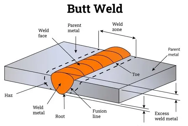
Example 2: Gaussian Heat Source for Butt Welding
Two rectangular plates are joined using a butt weld.
A moving Gaussian surface heat flux represents the welding arc.
The model can investigate how welding speed, heat input, and heat-source radius affect the temperature distribution.
Example 3: Goldak Double-Ellipsoidal Heat Source
The Goldak double-ellipsoidal heat source represents the volumetric distribution of heat around the welding arc.
The model uses separate front and rear ellipsoids.
Important parameters include:
- Front semi-axis
- Rear semi-axis
- Transverse semi-axis
- Depth parameter
- Heat-source efficiency
- Front and rear heat fractions
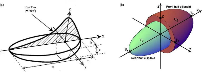
This model is particularly useful for arc welding simulations where a volumetric heat distribution is more appropriate than a simple surface Gaussian distribution.
Example 4: Goldak Heat Source for Butt-Welded Plates
A pair of plates is joined along a straight weld line.
The Goldak heat source moves through the weld region.
The model can be used to study:
- Weld penetration
- Thermal cycles
- Peak temperature
- Heat-affected zone
- Residual stress
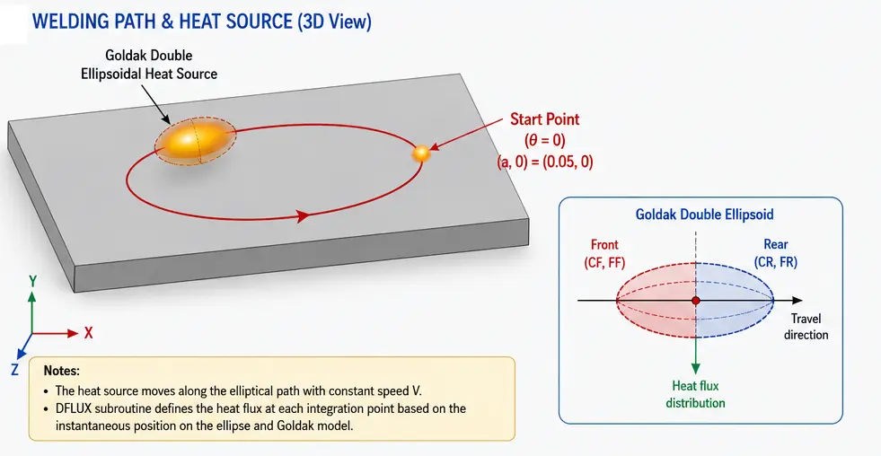
Example 5: Moving Heat Source Along an Elliptical Path
The welding torch follows an elliptical trajectory instead of a straight line.
The heat-source coordinates are defined using:
where (a_e) and (b_e) define the elliptical path.
This example is useful for curved welding paths and circumferential welding applications.
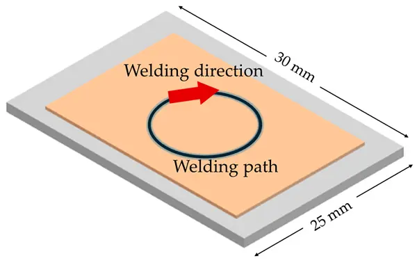
Example 6: Circular Welding Path
A moving heat source travels around a circular weld path.
The heat-source location changes continuously with time.
This model is useful for:
- Pipe welding
- Circular seams
- Cylindrical components
- Circumferential welding
Example 7: Welding Along an Arbitrary 3D Path
The heat source follows a user-defined three-dimensional trajectory.
Instead of using a simple analytical path, the welding coordinates can be supplied from a predefined path.
This approach is useful for complex industrial welds.
Example 8: TIG Welding Simulation
A TIG welding process is represented using a moving thermal source.
The model can investigate the effect of:
- Welding current
- Arc voltage
- Welding speed
- Heat-source efficiency
- Heat-source dimensions
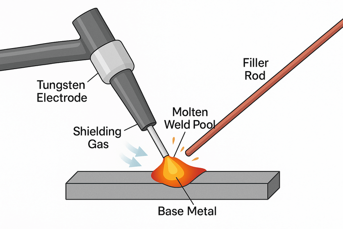
The electrical parameters can be converted into thermal power using an appropriate efficiency factor.
Example 9: MIG/MAG Welding Simulation
A moving heat source represents the thermal input from a MIG or MAG welding process.
The model can be used to investigate weld thermal cycles and residual stresses.
A more advanced model can incorporate filler-metal deposition and multiple weld passes.
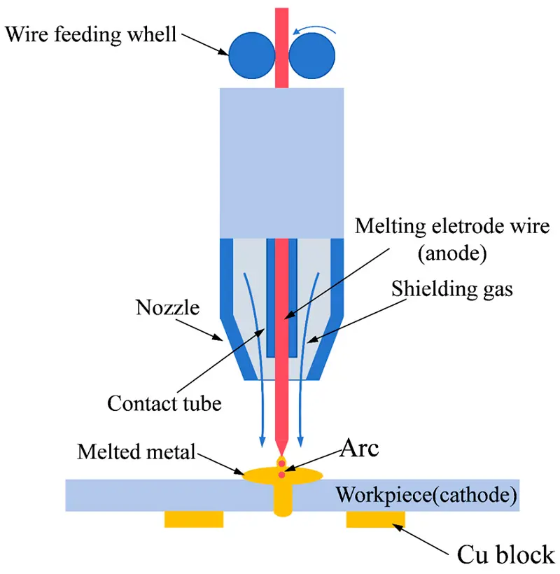
Example 10: Welding With Temperature-Dependent Convection
The welding simulation includes a convection coefficient that changes with temperature.
A FILM subroutine can define a temperature-dependent heat-transfer coefficient.
This is useful when a constant convection coefficient does not adequately represent the cooling process.
3. Laser Welding Simulation Examples
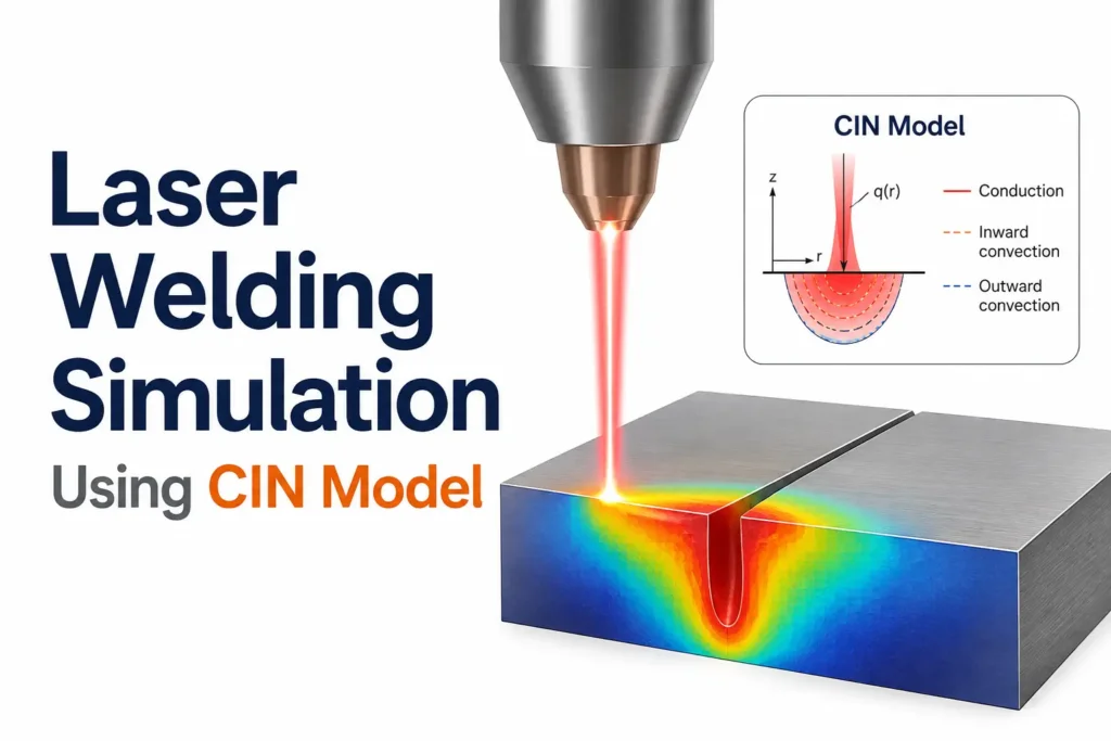
Laser welding produces a highly concentrated heat source.
Compared with conventional arc welding, laser welding often requires a smaller heat-source region and higher heat flux.
Example 11: Gaussian Laser Heat Source
A Gaussian distribution represents the laser intensity on the workpiece surface.
The heat flux can be expressed conceptually as:
where (R) represents a characteristic beam radius.
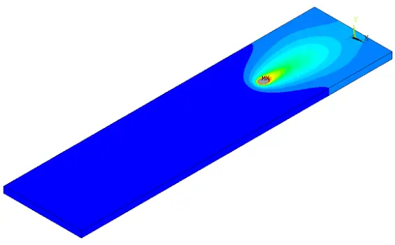
Example 12: Moving Laser Heat Source on a Plate
A laser heat source travels along a straight path.
The simulation predicts the transient thermal field and cooling history.
This is a useful starting point for laser welding FEA.
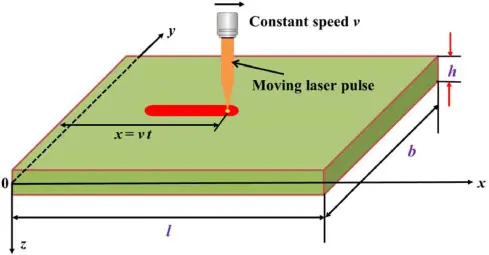
Example 13: Laser Welding of a Butt Joint
Two plates are joined using a moving laser heat source.
The simulation can evaluate:
- Peak temperature
- Thermal gradients
- Weld-zone temperature
- Heat-affected zone
- Cooling rate
Example 14: Laser Welding of Thin Sheets
A thin metal sheet is heated by a concentrated moving laser source.
Because the thickness is small, through-thickness thermal gradients can be particularly important.
Example 15: Laser Welding of a Cylindrical Component
A laser heat source moves around a cylindrical surface.
The heat-source coordinates must account for the curved geometry.
This provides a useful example of welding-path programming in Abaqus.
Example 16: Laser Welding With Radiation and Convection
The model includes both:
- Convective heat loss
- Radiative heat loss
The radiative heat flux can be represented by:
where:
- (\epsilon) is emissivity
- (\sigma) is the Stefan-Boltzmann constant
- (T) is the surface temperature
- (T_\infty) is ambient temperature
Example 17: Laser Welding With Temperature-Dependent Material Properties
Thermal conductivity, specific heat, density, and other material properties vary with temperature.
This produces a more realistic thermal response than a constant-property model.
4. Electron Beam Welding Examples
Electron beam welding uses a highly concentrated energy source.
The heat source can be represented using a localized surface or volumetric energy distribution.
Example 18: Moving Electron Beam Heat Source
A concentrated moving heat source travels along a plate.
The simulation predicts the transient temperature field.
Example 19: Electron Beam Butt Welding
Two plates are joined using a moving volumetric heat source.
The model can investigate the influence of beam power and travel speed.
Example 20: Deep-Penetration Electron Beam Model
A volumetric heat source is distributed through a relatively deep region.
This provides a simplified representation of deep-penetration welding.
5. Resistance Welding Examples
Resistance welding generates heat primarily through electrical resistance.
The basic physical relationship is:
where:
- (I) is current
- (R) is electrical resistance
- (t) is welding time
A detailed model can couple electrical, thermal, mechanical, and contact behavior.
Example 21: Resistance Spot Welding of Two Sheets
Two metal sheets are pressed between electrodes.
The model can investigate temperature development around the contact region.
Example 22: Resistance Spot Welding With Contact Pressure
Electrode pressure is included in the model.
This allows the simulation to investigate the relationship between contact pressure and thermal behavior.
Example 23: Resistance Spot Welding With Multiple Sheets
Three or more sheets are joined using resistance spot welding.
The model can evaluate temperature distribution through the stack.
Example 24: Thermo-Electro-Mechanical Resistance Welding
A more advanced model simultaneously considers:
- Electrical current
- Joule heating
- Temperature
- Mechanical deformation
- Contact behavior
This type of model is substantially more complex than a simple thermal welding model.
6. Friction Stir Welding Examples
Friction stir welding generates heat through friction and plastic deformation rather than an external arc.
The process involves a rotating tool moving along the joint.
Example 25: Simplified Friction Stir Welding Thermal Model
A moving thermal source represents the heat generated by the rotating tool.
This provides a relatively simple approach for predicting temperature fields.
Example 26: Rotating Heat Source for Friction Stir Welding
The heat input varies according to the rotating tool position.
The model can investigate the effect of rotational speed and travel speed.
Example 27: Friction Stir Welding of Butt Plates
Two plates are joined along a straight seam.
A moving heat source represents the thermal effect of the rotating tool.
Example 28: Friction Stir Welding With Mechanical Loading
The model includes tool-related mechanical loading in addition to the thermal field.
This allows investigation of:
- Contact pressure
- Plastic deformation
- Thermal expansion
- Residual stress
7. Pipe and Cylindrical Welding Examples
Pipe welding introduces additional geometric complexity because the welding path can follow a curved surface.
Example 29: Butt Welding of Two Pipes
Two cylindrical pipes are joined at their ends.
A moving heat source travels around the circumference.
Example 30: Circumferential Pipe Welding
A heat source moves continuously around a pipe.
This is an important Abaqus example for studying circumferential welding.
Example 31: Multi-Pass Pipe Welding
Several weld passes are deposited sequentially.
Each pass introduces additional heat into the pipe.
The simulation can predict the cumulative thermal history.
Example 32: Pipe Welding With Radiation and Convection
The model includes both radiation and convection from the external pipe surface.
This is useful for more realistic cooling predictions.
Example 33: Pipe-to-Plate Welding
A cylindrical pipe is welded to a flat plate.
The model can investigate the complex temperature distribution around the intersection.
Example 34: T-Joint Pipe Welding
A branch pipe is welded to a larger cylindrical pipe.
The geometry produces a curved weld path and nonuniform heat distribution.
8. Plate and Sheet-Metal Welding Examples
Flat plates provide relatively simple geometries for studying fundamental welding behavior.
Example 35: Single-Pass Plate Welding
A single weld pass travels across a rectangular plate.
The model predicts temperature distribution and thermal cycles.
Example 36: Double-Sided Welding
A weld is applied from both sides of the plate.
The second pass is applied after the first thermal cycle.
Example 37: Multi-Pass Plate Welding
Several weld passes are applied sequentially.
This model is useful for investigating the cumulative effects of repeated heating and cooling.
Example 38: Lap Joint Welding
Two overlapping sheets are joined using a moving heat source.
The model can investigate temperature gradients around the overlap region.
Example 39: T-Joint Welding
Two plates are joined at approximately 90 degrees.
A fillet-weld heat source is applied along the intersection.
Example 40: Cross-Welded Plates
Two weld paths intersect on the same plate.
The model can investigate thermal interaction between the welds.
9. Fillet Weld Simulation Examples
Fillet welds are common in structural and manufacturing applications.
Example 41: Single Fillet Weld
A simple T-joint contains one fillet weld.
The heat source moves along the joint.
Example 42: Double Fillet Weld
Both sides of a T-joint are welded sequentially.
The model can predict the combined thermal and mechanical effects.
Example 43: Fillet Weld With Welding Distortion
The thermal analysis is followed by a mechanical analysis.
Thermal expansion and contraction generate deformation.
The simulation can predict:
- Angular distortion
- Transverse displacement
- Longitudinal displacement
10. Thermal-Mechanical Welding Examples
A thermal analysis alone cannot predict welding distortion or residual stress.
A sequentially coupled thermal-mechanical approach is commonly used for these objectives.
Example 44: Sequential Thermal-Mechanical Welding Analysis
First, Abaqus calculates the transient temperature field.
The temperature history is then transferred to a mechanical analysis.
The mechanical model calculates:
- Thermal expansion
- Plastic deformation
- Residual stress
- Welding distortion
Example 45: Welding Residual Stress in a Plate
A moving heat source generates a transient thermal field.
The resulting temperature history drives a mechanical analysis.
The final stress state after cooling represents the predicted welding residual stress.
Example 46: Welding Distortion of a Thin Plate
A thin plate is welded along one edge.
The model predicts deformation after cooling to ambient temperature.
Thin plates are particularly useful for studying angular and out-of-plane distortion.
Example 47: Residual Stress in a Butt-Welded Joint
A butt-weld model is cooled from welding temperature to ambient conditions.
The final stress distribution is evaluated after the weld has cooled.
Example 48: Thermal Stress Around a Weld
The model focuses on the stress generated by nonuniform thermal expansion.
The highest stresses generally occur near strong temperature gradients and constrained regions.
11. Fully Coupled Temperature-Displacement Welding Examples
Instead of separating the thermal and mechanical analyses, Abaqus can also solve temperature and displacement degrees of freedom together when the physical problem and element formulation are appropriate.
Example 49: Fully Coupled Welding of a Constrained Plate
The plate is mechanically constrained while a moving heat source is applied.
The simulation simultaneously evaluates temperature and deformation.
Example 50: Thermo-Mechanical Welding of a Thin Sheet
A thin sheet experiences rapid heating and cooling.
The fully coupled analysis accounts for the interaction between temperature and deformation.
12. Multi-Pass Welding and Element Activation
Multi-pass welding is considerably more realistic than a single-pass model for many engineering applications.
Example 51: Two-Pass Welding Simulation
Two separate heat-source paths are applied sequentially.
The second pass reheats material affected by the first pass.
Example 52: Three-Pass Welding Simulation
Three weld passes are activated sequentially.
The model can investigate the accumulation of thermal cycles.
Example 53: Multi-Pass Welding With Element Activation
Elements representing weld material are activated according to the welding sequence.
This provides a way to approximate progressive weld deposition.
Example 54: Multi-Layer Additive Welding
Multiple material layers are deposited sequentially.
Each deposited layer receives a moving heat input.
This type of model is closely related to Wire Arc Additive Manufacturing.
13. Welding Simulation With User Subroutines
User subroutines provide substantial flexibility for welding simulations.
Example 55: DFLUX Moving Heat Source
A DFLUX subroutine defines a spatially and temporally varying heat flux.
The heat source position can depend on:
- Time
- Node coordinates
- Element coordinates
- Welding speed
- Welding path
A DFLUX-based model is one of the most useful approaches for customized welding simulations in Abaqus.
Example 56: DFLUX Gaussian Heat Source
The DFLUX subroutine applies a Gaussian heat distribution that moves along a predefined welding path.
This is suitable for laser and simplified arc-welding models.
Example 57: DFLUX Goldak Heat Source
The DFLUX implementation calculates the front and rear components of a double-ellipsoidal heat source.
The source moves according to the welding direction.
This provides a flexible implementation of the Goldak model.
Example 58: FILM Subroutine for Temperature-Dependent Convection
The FILM subroutine defines a convection coefficient that varies with temperature.
This can improve the representation of cooling from the welded component.
Example 59: Welding Heat Source Along a Custom Path
A user-defined path controls the location of the heat source.
The path can be:
- Straight
- Circular
- Elliptical
- Helical
- Piecewise
- Three-dimensional
This approach is useful for complex welding trajectories.
Example 60: User-Defined Welding Heat Input
A custom subroutine controls heat input as a function of time and position.
This allows the model to reproduce experimentally measured or machine-specific welding power profiles.
14. Welding Simulation Examples by Heat-Source Type
The same welding process can be modeled using different heat-source formulations.
| Heat Source | Typical Application | Main Advantage |
|---|---|---|
| Gaussian | Laser, arc welding | Simple and computationally efficient |
| Goldak double ellipsoid | Arc welding | Represents front/rear volumetric heat distribution |
| Point source | Simplified models | Very easy to implement |
| Line source | Thin structures | Simple distributed heating |
| Surface heat flux | Laser/arc | Convenient for surface heating |
| Body heat flux | Deep penetration | Represents volumetric energy deposition |
| User-defined source | Complex welding | Maximum flexibility |
| Moving source | Most welding processes | Represents torch/tool movement |
Choosing the correct heat-source model is critical.
15. FAQ: Abaqus Welding Simulation
What is Abaqus welding simulation?
Abaqus welding simulation uses finite element analysis to calculate the thermal and mechanical response of a component during and after welding.
It can predict temperature, thermal cycles, residual stress, plastic deformation, and welding distortion.
Which Abaqus subroutine is commonly used for welding heat sources?
DFLUX is commonly used to define a spatially and temporally varying heat flux.
It is particularly useful for moving welding heat sources.
What is the Goldak heat source?
The Goldak model is a double-ellipsoidal volumetric heat-source model commonly used to represent arc welding heat input.
It uses separate front and rear heat-source regions.
What is the difference between Gaussian and Goldak heat sources?
A Gaussian heat source commonly represents a surface or localized radial heat distribution.
The Goldak model represents a three-dimensional volumetric distribution with separate front and rear regions.
The appropriate choice depends on the welding process and available experimental data.
Can Abaqus predict welding residual stress?
Yes.
A thermal analysis can generate the temperature history, which can then drive a mechanical analysis to calculate residual stresses after cooling.
Can Abaqus predict welding distortion?
Yes.
A thermo-mechanical model can calculate deformation caused by nonuniform thermal expansion, plasticity, and cooling.
Is radiation important in welding simulation?
It can be.
Radiation becomes increasingly significant as surface temperature increases. Its importance depends on the process, temperature range, surface properties, and surrounding environment.
Can Abaqus simulate multi-pass welding?
Yes.
A multi-pass welding model can apply multiple heat-source paths sequentially. Element activation can also be used to represent progressive weld deposition.
Can Abaqus simulate laser welding?
Yes.
A moving Gaussian or other appropriate heat-source formulation can be used to represent laser energy input.
Can Abaqus simulate pipe welding?
Yes.
Pipe welding can be modeled using a moving heat source following a circumferential or other three-dimensional welding path.
What is the best Abaqus element for welding simulation?
There is no single best element for every welding problem.
The element must match the analysis type. Thermal simulations require elements with temperature degrees of freedom, while sequential thermo-mechanical analyses require suitable thermal and mechanical formulations for their respective steps.
How do I validate an Abaqus welding simulation?
Compare predictions against experimental measurements such as:
- Thermocouple temperature histories
- Weld dimensions
- Thermal cycles
- Distortion measurements
- Residual stress measurements
- Hardness or microstructure data
Validation should be performed before using the model for engineering predictions.
16. Conclusion
Abaqus provides a flexible platform for developing welding simulations ranging from simple moving heat-source models to advanced thermo-mechanical and multi-pass welding analyses.
The most important components of an Abaqus welding simulation are usually:
- An appropriate heat-source model
- Correct welding speed
- Realistic heat input
- Temperature-dependent material properties
- Appropriate convection and radiation
- Adequate mesh resolution
- Correct welding sequence
- Appropriate thermal and mechanical boundary conditions
- Experimental validation
For beginners, the best starting point is a transient thermal analysis of a flat plate with a moving Gaussian heat source.
Once that model works correctly, you can progress to DFLUX, Goldak heat sources, curved welding paths, radiation, temperature-dependent properties, multi-pass welding, residual stress, and welding distortion.
For advanced projects, the same methodology can be extended to pipe welding, laser welding, electron beam welding, resistance welding, friction stir welding, and multi-layer deposition.
The 60 examples in this guide provide a structured roadmap for developing increasingly sophisticated Abaqus FEA welding simulations.
If your goal is engineering consulting, academic research, or building a reusable Abaqus project library, these examples can also be organized into dedicated categories such as Abaqus Welding Tutorials, Welding CAE Models, DFLUX Subroutines, Goldak Heat Sources, Multi-Pass Welding, Welding Residual Stress, and Welding Distortion.