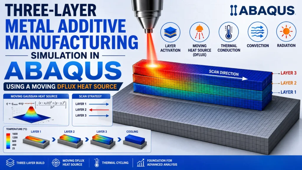
In this tutorial, we develop a simple three-layer metal additive manufacturing model in Abaqus. The model uses a thin wall deposited on a metallic substrate and a moving Gaussian heat source implemented with the DFLUX user subroutine.
The model focuses on the essential thermal behavior of additive manufacturing, including layer activation, localized heat input, thermal conduction, repeated heating and cooling, and final cooling.
The goal is to provide a simple and computationally efficient starting point for understanding thermal behavior before progressing to more advanced simulations of melt-pool dynamics, residual stress, and distortion.
1- Simulation Summary – Three-Layer Metal Additive Manufacturing
A simplified Abaqus thermal model using progressive layer activation, a moving Gaussian DFLUX heat source, thermal conduction, convection, and radiation.
Simulation Workflow
Temperature
Model Geometry
| Substrate | 100 × 50 × 6 mm |
| Wall length | 50 mm |
| Wall thickness | 3 mm |
| Layer height | 3 mm |
| Number of layers | 3 |
Process Parameters
| Material | 316L Stainless Steel |
| Laser power | 1000 W |
| Absorptivity | 0.35 |
| Scan speed | 5 mm/s |
| Beam radius | 1 mm |
Abaqus Model Components
Progressive activation of the deposited layers.
Moving Gaussian heat source.
Heat transfer through the wall and substrate.
Heat loss to the surrounding environment.
High-temperature radiative heat loss.
Layer-by-Layer Deposition Strategy
Typical Thermal Cycling
A point in a previously deposited layer can be reheated when subsequent layers are deposited.
Note: The graph is illustrative and represents the expected repeated heating and cooling behavior. It is not experimental temperature data.
Key Takeaway
This three-layer Abaqus model provides a simple foundation for metal additive manufacturing FEA. It combines progressive layer activation, a moving DFLUX heat source, thermal conduction, convection, and radiation. The resulting thermal history can later be transferred to a mechanical analysis to investigate residual stress and distortion.
The alternating scan direction represents a simple bidirectional deposition strategy.
The complete analysis consists of:
- Initial temperature assignment
- Deposition of Layer 1
- Deposition of Layer 2
- Deposition of Layer 3
- Final cooling
The thermal analysis predicts the temperature field throughout the deposition process.
2. Geometry
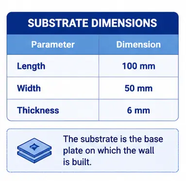
The substrate is modeled as a rectangular block.
Substrate Dimensions
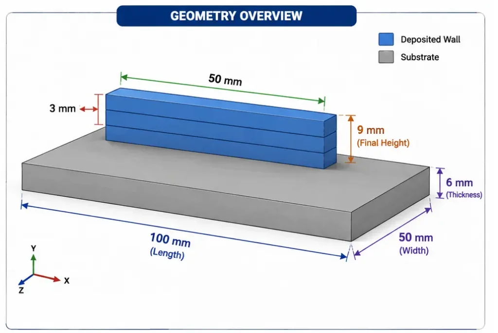
A thin wall is deposited on the upper surface of the substrate.
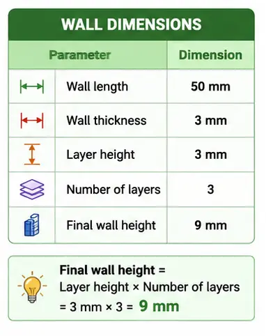
Wall Dimensions for MA Simulation
Geometric parameters used for the three-layer metal additive manufacturing simulation.
The wall is positioned approximately at the center of the substrate.
The three layers are partitioned separately so that each layer can be activated and heated independently.
             Layer 3
        ┌──────────────┐
        │              │
        ├──────────────┤
             Layer 2
        ├──────────────┤
             Layer 1
        └──────────────┘
        ████████████████
            Substrate
3. Material Selection
For this simplified example, both the substrate and deposited material are assumed to be 316L stainless steel.
Using the same material for the substrate and deposited layers keeps the model simple and allows us to focus on the additive manufacturing process itself.
The thermal material definition requires:
📌 Note: For a preliminary demonstration, a density of approximately 8000 kg/m³ can be used.
⚠️ Important: A serious engineering simulation should use temperature-dependent thermal properties obtained from reliable experimental or literature data.
4. Thermal Finite Element Type
The analysis is a transient heat-transfer problem.
Therefore, heat-transfer elements should be used.
A suitable element is:
DC3D8 — 8-node linear heat transfer brick
The mesh should be refined around the deposited wall and the expected heat-source path.
A mesh size of approximately 1 mm can be used as an initial value near the deposition region.
A mesh convergence study should be performed before using the model for quantitative engineering predictions.
5. Layer Partitioning
The wall is divided into three independent layers.
The layer sets can be named:
LAYER_1
LAYER_2
LAYER_3
Separating the layers is important because each layer is activated during a different deposition step.
6. Layer Activation
The additive manufacturing process is represented by progressively activating the deposited material.
Initially, only the substrate and the first layer participate in the simulation.
After the first deposition pass, Layer 2 becomes active.
After the second pass, Layer 3 becomes active.
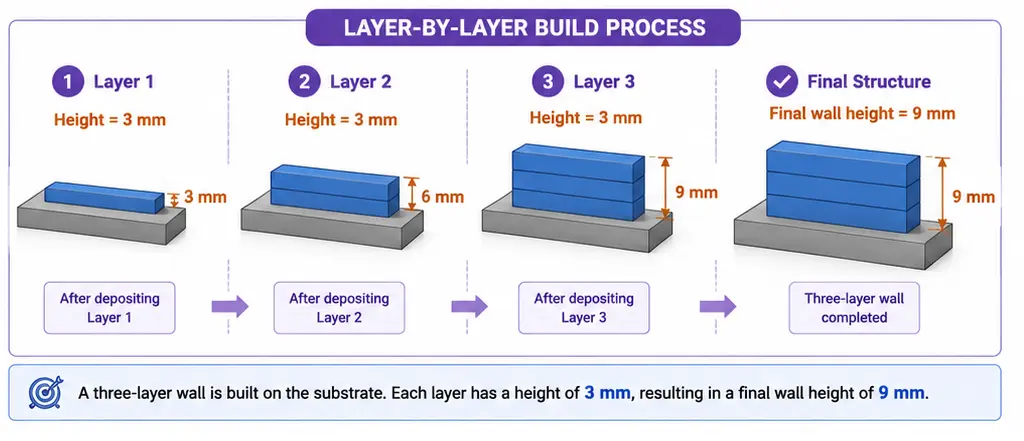
Conceptually:
Step 1

Layer 3   inactive
Layer 2   inactive
Layer 1   ACTIVE
Substrate ACTIVE
Then:
Step 2

Layer 3   inactive
Layer 2   ACTIVE
Layer 1   ACTIVE
Substrate ACTIVE
Finally:
Step 3

Layer 3   ACTIVE
Layer 2   ACTIVE
Layer 1   ACTIVE
Substrate ACTIVE
This progressive activation is one of the fundamental concepts in finite element modeling of additive manufacturing.
The exact activation implementation depends on the Abaqus workflow. Element activation can be controlled using appropriate model-change or element-activation techniques.
7. Initial Temperature
The initial temperature of the substrate and inactive material is assumed to be:
This represents a room-temperature substrate.
The actual process may use substrate preheating. If experimental data are available, the model should use the real build-plate temperature instead.
The initial temperature can be assigned using a predefined temperature field in Abaqus.
8. Moving Heat Source
Instead of assigning a fixed temperature to each layer, a moving heat source is used.
This is a more physically meaningful representation of laser-based deposition.
The heat source travels along the wall:
Layer 1:
Laser ─────────────→

Layer 2:
Laser ←─────────────

Layer 3:
Laser ─────────────→
The heat source is implemented using the Abaqus DFLUX user subroutine.
9. Gaussian Heat Source
A simple surface Gaussian heat source can be expressed as:
Applied heat flux.
Maximum heat flux at the center of the heat source.
Current laser position along the scan direction.
Centerline of the deposited wall.
Effective radius of the laser heat source.
Moving Heat Source
The laser position changes continuously with time as the heat source travels along the deposited layer.
Three-Layer Scan Strategy
10. Suggested Heat-Source Parameters
For this introductory model, the following values can be used as starting parameters:
| Parameter | Value |
| Laser power | 1000 W |
| Absorptivity | 0.35 |
| Absorbed power | 350 W |
| Scan speed | 5 mm/s |
| Beam radius | 1 mm |
The absorbed laser power is:
With an absorptivity of η = 0.35 and a laser power of P = 1000 W, the model applies an absorbed power of 350 W.
These values are intended for a demonstration model, not as experimentally validated processing parameters for 316L.
In a research model, the laser power, absorptivity, beam radius, and scan speed should be calibrated against experimental temperature or melt-pool measurements.
11. Deposition Time
The wall has a deposition length of:
The laser velocity is:
Therefore, the time required to scan one layer is:
Thus, each layer is deposited during a 10-second analysis step.
The deposition sequence is:
| Step | Layer | Scan direction | Time |
| 1 | Layer 1 | Forward | 10 s |
| 2 | Layer 2 | Reverse | 10 s |
| 3 | Layer 3 | Forward | 10 s |
| 4 | Cooling | — | 30–60 s |
The total active deposition time is:
12. DFLUX Implementation
The DFLUX subroutine calculates the Laser heat flux at integration points on the surface where the heat source is applied.
The basic logic is:
Step 1:
Laser moves from xmin to xmax

Step 2:
Laser moves from xmax to xmin

Step 3:
Laser moves from xmin to xmax
The current step time is used to calculate the laser position.
For example, for Layer 1:
For Layer 2:
For Layer 3:
This allows the laser to restart from the correct position at the beginning of each deposition step.
A critical point in DFLUX implementation is to handle the step time correctly. Using total analysis time without considering the current step can cause the heat source to start from the wrong location in subsequent layers.
13. Convection
The exposed surfaces lose heat through convection.
The convection heat flux is:
For the initial model, use:
and:
Apply convection to the exposed surfaces of the substrate and deposited wall.
Do not apply convection to internal interfaces between the substrate and deposited material.
14. Radiation
Radiation is also included because the deposition region reaches high temperatures.
The radiative heat flux is:
where:
- (\epsilon) is surface emissivity,
- (\sigma) is the Stefan–Boltzmann constant,
- (T) is the absolute surface temperature,
- (T_\infty) is the absolute ambient temperature.
A starting emissivity of:
can be used for the demonstration.
The ambient temperature is:
When calculating radiation, temperatures must be treated as absolute temperatures in Kelvin.
15. Thermal Interaction Between Layers
The deposited layers should conduct heat to each other.
If the layers are constructed as a conformal mesh with shared nodes, heat conduction occurs naturally through the common interface.
The model therefore does not require mechanical contact or friction.
The thermal path is:
Laser
  ↓
Layer 3
  ↓
Layer 2
  ↓
Layer 1
  ↓
Substrate
  ↓
Build plate
This conductive heat transfer is essential because newly deposited material reheats the previously deposited layers.
16. Substrate Boundary Condition
The bottom of the substrate acts as a heat sink.
For this simplified model, the bottom surface can be maintained at:
This provides a simple and stable thermal boundary condition.
However, this assumption can remove heat too aggressively compared with a real manufacturing system.
A more realistic model could represent the build plate using:
- Contact conductance
- A separate build-plate model
- Temperature-dependent boundary conditions
- Experimental substrate temperature data
For the first model, a prescribed bottom temperature is sufficient.
17. Mechanical Boundary Conditions
The current analysis is thermal, so mechanical constraints are not required.
If the thermal model is later coupled to a mechanical analysis, appropriate mechanical constraints must be applied to represent the substrate fixture.
For example, the bottom of the substrate can be constrained against rigid-body motion.
Care should be taken not to over-constrain the substrate because excessive constraints can produce unrealistic residual stresses.
18. Analysis Steps in Abaqus
A practical Abaqus step structure is:
Initial Step
Assign:
to the model.
Step 1 – Deposition of Layer 1
- Activate Layer 1
- Apply DFLUX
- Scan from left to right
- Duration: 6 s
- Convection active
- Radiation active
Step 2 – Deposition of Layer 2
- Activate Layer 2
- Restart laser position
- Scan from right to left
- Duration: 10 s
- Convection active
- Radiation active
Step 3 – Deposition of Layer 3
- Activate Layer 3
- Restart laser position
- Scan from left to right
- Duration: 10 s
- Convection active
- Radiation active
Step 4 – Cooling
- Remove DFLUX
- Keep convection active
- Keep radiation active
- Duration: 30–60 s
This final cooling step is important because the temperature field immediately after deposition is not the final thermal state.
19. Important Abaqus Interactions
The thermal model should contain:
Convection
Film condition on exposed surfaces.
Radiation
Surface radiation to ambient.
Thermal conduction
Naturally through connected elements.
You generally do not need:
- General contact
- Friction
- Mechanical contact
- Tie constraints between conformal layers
if the wall and substrate use a compatible connected mesh.
If separate parts are used, an appropriate thermal tie/coupling method must be introduced.
20. Recommended Output Variables
The most important output is temperature:
NT11
Request NT11 as a field output.
You can then visualize:
- Temperature contour
- Maximum temperature
- Heat-affected region
- Cooling behavior
Other useful thermal outputs include heat flux and energy-related quantities where appropriate.
It is also useful to create history output at selected points.
For example:
Point A → near Layer 1
Point B → near Layer 2
Point C → near Layer 3
The resulting temperature histories should show repeated heating.
21. Expected Thermal Behavior
The temperature field should show a highly localized hot region around the moving heat source.
During Layer 1 deposition:
        🔥
───────────────
Layer 1
═══════════════
Substrate
After the laser moves away, the region cools.
When Layer 2 is deposited, heat flows downward into Layer 1 and the substrate.
Therefore, a point located in Layer 1 can experience:
Temperature
    ↑
    │        /\
    │       /  \       ← Layer 2 reheating
    │  /\  /    \
    │ /  \/      \__
    └────────────────→ Time
       L1    L2
When Layer 3 is deposited, the same region may experience another thermal cycle.
This repeated reheating is one of the most important phenomena demonstrated by the model.
22. What Should Be Checked After the Simulation?
Before trusting the results, check the following.
Check 1 – Does the heat source move?
Create an animation of NT11.
The high-temperature region should clearly travel along the wall.
Check 2 – Does the laser reverse direction?
Layer 1 should scan:
left → right
Layer 2:
right → left
Layer 3:
left → right
Check 3 – Does each layer activate at the correct time?
Layer 2 should not behave as an active deposited layer during Step 1.
Check 4 – Does temperature decrease during cooling?
After removing DFLUX, the wall should progressively cool toward ambient temperature.
Check 5 – Is the temperature physically reasonable?
An extremely high temperature can indicate excessive heat input, incorrect units, incorrect DFLUX implementation, or inappropriate material properties.
23. Why This Is a Useful Abaqus Example
This three-layer model is deliberately simple, but it contains the fundamental components required for a more advanced metal additive manufacturing simulation:
It also demonstrates the most important computational concept in AM FEA:
Once this model has been verified, it can be extended to five, ten, or hundreds of layers
24. Possible Extensions
The model can be upgraded progressively.
Extension 1 – Temperature-dependent properties
Replace constant thermal conductivity and specific heat with experimentally measured temperature-dependent data.
Extension 2 – More layers
Increase the wall from three layers to:
- 5 layers
- 10 layers
- 20 layers
- 50 layers
Extension 3 – Different scanning strategies
Compare:
- Unidirectional scanning
- Bidirectional scanning
- Rotated scan directions
- Different scan speeds
Extension 4 – Temperature-dependent convection
A FILM subroutine can be introduced to make the convection coefficient dependent on temperature.
Extension 5 – Thermomechanical analysis
Transfer the temperature history into a mechanical model to calculate:
- Thermal stress
- Plastic strain
- Residual stress
- Distortion
Extension 6 – Multi-material deposition
The model can eventually be extended to dissimilar materials such as H13 and Inconel 718.
25. Limitations of the Simplified Model
This model should not be interpreted as a complete melt-pool simulation.
It does not explicitly model:
- Melt-pool fluid flow
- Surface tension
- Marangoni convection
- Evaporation
- Powder dynamics
- Solidification microstructure
- Phase transformations
- Keyhole formation
- Metal vaporization
The Gaussian DFLUX model is an engineering approximation of the heat input.
Therefore, quantitative predictions should be validated against experimental measurements.
The most important parameters to calibrate are:
- Laser power
- Absorptivity
- Scan speed
- Beam radius
- Thermal properties
- Convection coefficient
- Emissivity
26. Conclusion
A three-layer thin-wall model provides an excellent starting point for learning metal additive manufacturing simulation in Abaqus.
The model combines progressive layer activation with a moving Gaussian heat source implemented through DFLUX. Convection and radiation provide heat-loss mechanisms, while the substrate provides a conductive heat sink.
The complete process can be summarized as:
The resulting temperature history demonstrates localized heating, heat conduction, cooling, and reheating of previously deposited material.
This three-layer benchmark can then serve as the foundation for a more advanced thermomechanical Abaqus model for residual stress and distortion prediction.
For researchers and engineers learning additive manufacturing FEA, starting with a small validated model is preferable to immediately building a large multi-layer simulation with complicated physics. Once the heat source, material data, activation strategy, and thermal boundary conditions are verified, the model can be expanded systematically.