Composite 4-layer plate simulation in Abaqus

Here’s an example of simulating a 4-layer composite plate in Abaqus with dimensions 1 m × 0.5 m × 0.001 m. The plate is made of a carbon fiber-epoxy composite, and we will define the stacking sequence as [0°, 45°, -45°, 90°]. Each ply has a thickness of 0.00025 m (total thickness = 0.001 m).

Theory of Composite Laminated Plate Analysis

Composite laminated plates are structures made by stacking multiple layers (plies) of fiber-reinforced materials bonded together. Each layer can have a distinct fiber orientation, material properties, and thickness. Solving composite plate problems involves understanding the mechanics of anisotropic materials, laminate theory, and failure criteria.

1. Key Assumptions

1. Classical Laminated Plate Theory (CLPT):
   • Based on Kirchhoff-Love hypotheses (similar to thin plate theory).
   • Straight lines normal to the mid-surface remain straight and normal after deformation.
   • Transverse shear strains are neglected (γxz=γyz=0γxz​=γyz​=0).
2. First-Order Shear Deformation Theory (FSDT):
   • Accounts for transverse shear deformation.
   • Relaxes the normality assumption (lines remain straight but not necessarily normal).
3. Material Behavior:
   • Each ply is orthotropic (different properties in principal directions).
   • Linear elastic behavior within each layer.

2. Laminate Configuration

Definition:

• Stacking Sequence: Fiber orientations of each ply (e.g., $[0°,45°,-45°,90°]$).
• Ply Thickness: tktk​ for the $k$-th layer.
• Material Properties: For each ply:
  • Longitudinal modulus (E1E1​),
  • Transverse modulus (E2E2​),
  • Shear modulus (G12G12​),
  • Poisson’s ratios (ν12,ν21ν12​,ν21​).

3. Constitutive Equations

For a Single Ply (Orthotropic Material)

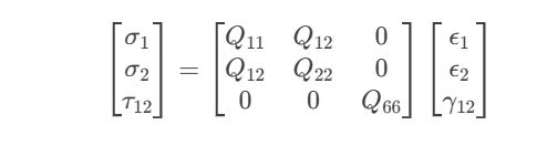
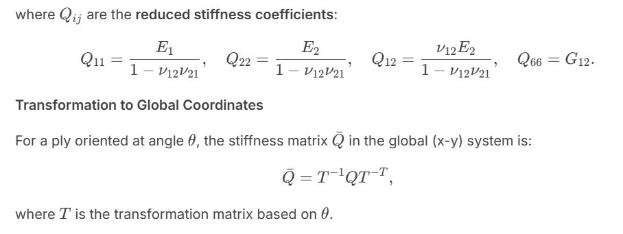
The stress-strain relationship in the material coordinate system (1-2) is:

4. Laminate Stiffness Matrix (ABD Matrix)

The ABD matrix relates forces/moments to mid-plane strains/curvatures:

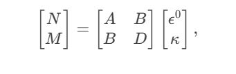
where:

• $N$: In-plane force resultants.
• $M$: Moment resultants.
• ϵ0ϵ0: Mid-plane strains.
• $\kappa$: Curvatures.
• $A,B,D$: Extensional, coupling, and bending stiffness matrices.

Calculation of $A,B,D$:

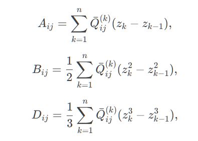
where zkzk​ is the distance from the mid-plane to the top of the $k$-th ply.

5. Governing Equations

Using equilibrium and strain-displacement relationships, the governing equations for a laminated plate are derived. For CLPT:

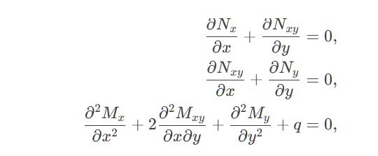
where $q$ is the transverse load.

6. Solution Methods

1. Analytical Solutions:
   • Applicable for simple geometries and boundary conditions (e.g., simply supported rectangular plates).
   • Use Navier or Lévy methods to solve the governing equations.
2. Numerical Methods (FEA):
   • Discretize the plate into shell elements (e.g., S4R in Abaqus).
   • Solve using the finite element method (FEM).

7. Failure Analysis of Composite laminates 

Failure reasons:

• Fiber Failure: Tensile/compressive failure along the fiber direction.
• Matrix Failure: Cracking or shear failure in the matrix.
• Delamination: Separation between plies.

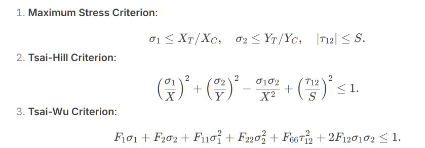
Failure Criteria:

1. Maximum Stress Criterion:

8. Example Problem

Problem: A 4-ply symmetric laminate $[0°/45°/-45°/90°]$ with dimensions $1\text{m}\times 0.5\text{m}\times 0.001\text{m}$ is subjected to a uniform pressure load. Calculate the deflection and stresses.

Steps:

1. Compute the ABD matrix using ply properties.
2. Solve the governing equations using FEA (e.g., Abaqus).
3. Extract mid-plane strains and curvatures.
4. Compute ply stresses using the transformed stiffness matrices.
5. Apply failure criteria to check for ply failure.

9. Practical Implementation in Abaqus

• Use shell elements with composite section definitions.
• Define material orientations for each ply.
• Specify stacking sequence and ply thicknesses.
• Apply loads and boundary conditions.
• Post-process results to evaluate stresses, strains, and failure indices.

Step-by-Step Example of 4-layer composite plate in Abaqus

1. Problem Setup

• Dimensions: 1 m (length) × 0.5 m (width) × 0.001 m (thickness).
• Material: Carbon Fiber-Epoxy (orthotropic material).
  • E1=230 GPaE1​=230 GPa (longitudinal modulus).
  • E2=15 GPaE2​=15 GPa (transverse modulus).
  • ν12=0.3ν12​=0.3 (Poisson’s ratio).
  • G12=50 GPaG12​=50 GPa (shear modulus).
• Stacking Sequence: $[0°,45°,-45°,90°]$.
• Ply Thickness: 0.00025 m per ply (4 plies total).

2. Step-by-Step Procedure

Step 1: Launch Abaqus/CAE

1. Open Abaqus/CAE.
2. Create a new model database.

Step 2: Create the Geometry

1. Create a Part:
   • Go to Part Module.
   • Click Create Part.
   • Name: Composite_Plate, Type: 3D Deformable, Base Feature: Shell.
   • Approximate size: 1.2.
   • Draw a rectangle with Length = 1 m and Width = 0.5 m.
   • Assign Thickness = 0.001 m.

Step 3: Define Material Properties

1. Create Material:
   • Go to Property Module.
   • Click Create Material, name: Carbon_Fiber_Epoxy.
   • Under Mechanical > Elastic, select Lamina (for orthotropic material).
   • Enter material properties:
     • E1=230e9 PaE1​=230e9 Pa, E2=15e9 PaE2​=15e9 Pa, ν12=0.3ν12​=0.3, G12=50e9 PaG12​=50e9 Pa, G13=50e9 PaG13​=50e9 Pa, G23=5e9 PaG23​=5e9 Pa.
2. Define Ply Orientations:
   • Create a Layup:
     • Click Create Composite Layup, name: Composite_Layup.
     • Assign the material Carbon_Fiber_Epoxy.
     • Define the stacking sequence:
       • Ply 1: 0°, Thickness = 0.00025 m.
       • Ply 2: 45°, Thickness = 0.00025 m.
       • Ply 3: -45°, Thickness = 0.00025 m.
       • Ply 4: 90°, Thickness = 0.00025 m.

Step 4: Assign Section and Layup

1. Create Section:
   • Click Create Section, name: Composite_Section.
   • Category: Shell, Type: Composite.
   • Assign the composite layup: Composite_Layup.
2. Assign Section to Part:
   • Select the plate geometry.
   • Click Assign Section and choose Composite_Section.

Step 5: Mesh the Model

1. Seed the Part:
   • Go to Mesh Module.
   • Click Seed Part, approximate global size: 0.05 m.
2. Assign Element Type:
   • Click Assign Element Type.
   • Family: Shell, Element Type: S4R (4-node reduced-integration shell element).
3. Generate Mesh:
   • Click Mesh Part to generate the mesh.

Step 6: Define Boundary Conditions for Composite Plate

1. Apply Constraints:
   • Go to Load Module.
   • Assume the plate is clamped on one edge:
     • Click Create Boundary Condition, name: Fixed_Edge.
     • Select the edge to fix and constrain all degrees of freedom (U1, U2, U3, UR1, UR2, UR3).

Step 7: Apply Loads to Composite Plate

1. Apply Mechanical Load:
   • Click Create Load, name: Pressure_Load.
   • Select the top surface of the plate.
   • Apply a uniform pressure (e.g., 1000 Pa).

Step 8: Create a Static Step

1. Create Step:
   • Go to Step Module.
   • Click Create Step, name: Static_Step, Procedure: Static, General.

Step 9: Submit the Job for Composite Plate Analysis

1. Create Job:
   • Go to Job Module.
   • Click Create Job, name: Composite_Plate_Analysis.
   • Submit the job.
2. Run the Analysis:
   • Click Submit and monitor the job status.
   • Check the .dat file for errors.

Step 10: Post-Processing

1. Open Results:
   • Go to Visualization Module.
   • Open the output database (Composite_Plate_Analysis.odb).
2. Plot Deformation and Stresses:
   • Click Plot > Deformed Shape to visualize deformation.
   • Use Plot > Contour to plot stress distributions (e.g., von Mises stress, principal stresses).
3. Extract Results:
   • Go to Report > Field Output.
   • Select variables (e.g., stress, strain) and save the report.

3. Example Python Script for Automation

from abaqus import *
from abaqusConstants import *
from caeModules import *

# Create model and part
mdb.Model(name='Composite_Plate')
myModel = mdb.models['Composite_Plate']
myPart = myModel.Part(name='Plate', dimensionality=THREE_D, type=DEFORMABLE_SHELL)
mySketch = myModel.ConstrainedSketch(name='Sketch', sheetSize=1.2)
mySketch.rectangle(point1=(0,0), point2=(1,0.5))
myPart.BaseShell(sketch=mySketch)

# Define composite material
myMaterial = myModel.Material(name='Carbon_Fiber_Epoxy')
myMaterial.Elastic(type=LAMINA, table=((230e9, 15e9, 0.3, 50e9, 50e9, 5e9), ))

# Define composite layup
myCompositeLayup = myModel.CompositeLayup(name='Composite_Layup', description='4-ply laminate')
myCompositeLayup.CompositePly(suppressed=False, plyName='Ply-1', region=myPart.Set(faces=myPart.faces), 
    material='Carbon_Fiber_Epoxy', thickness=0.00025, orientation=0.0)
myCompositeLayup.CompositePly(suppressed=False, plyName='Ply-2', region=myPart.Set(faces=myPart.faces), 
    material='Carbon_Fiber_Epoxy', thickness=0.00025, orientation=45.0)
myCompositeLayup.CompositePly(suppressed=False, plyName='Ply-3', region=myPart.Set(faces=myPart.faces), 
    material='Carbon_Fiber_Epoxy', thickness=0.00025, orientation=-45.0)
myCompositeLayup.CompositePly(suppressed=False, plyName='Ply-4', region=myPart.Set(faces=myPart.faces), 
    material='Carbon_Fiber_Epoxy', thickness=0.00025, orientation=90.0)

# Mesh
myPart.seedPart(size=0.05)
myPart.setElementType(elemTypes=(ElemType(elemCode=S4R, elemLibrary=STANDARD), ))
myPart.generateMesh()

# Boundary conditions
myModel.DisplacementBC(name='Fixed_Edge', createStepName='Initial', region=myPart.Set(edges=myPart.edges[0]), 
    u1=SET, u2=SET, u3=SET, ur1=SET, ur2=SET, ur3=SET)

# Load
myModel.Pressure(name='Pressure_Load', createStepName='Static_Step', region=myPart.Set(faces=myPart.faces), 
    magnitude=1000.0)

# Step
myModel.StaticStep(name='Static_Step', previous='Initial')

# Job
myJob = mdb.Job(name='Composite_Plate_Analysis', model='Composite_Plate')
myJob.submit()
myJob.waitForCompletion()

Read more:

Effect of glass fiber reinforced polymer composite material

Structure, mechanical properties, and finite-element modeling of an Al particle/resin composite