Natural Frequency Analysis of a Sheet in Abaqus

By understanding the concepts, engineers can predict vibrational behavior, avoid resonance, and optimize designs in fields ranging from civil engineering to aerospace.

• Natural frequencies are intrinsic properties of a system governed by mass, stiffness, and boundary conditions.
• Mode shapes: The dynamic deflection shape of linear structures can be decomposed in a sum of elementary vibration patterns. These vibration patterns are called mode shapes, they are illustrated below with the example of a cantilever beam.

Natural Frequency Theory and Mode Shapes

1. Natural Frequency

Definition:
Natural frequency is the rate at which a body vibrates when disturbed without being subject to a driving or damping force. The pattern or shape of this vibrating motion is the corresponding mode of the body’s or system’s vibration, known as the normal mode

Key Characteristics:

• Each system has multiple natural frequencies, corresponding to different vibrational patterns (mode shapes).
• Natural frequencies depend on:
  • Mass distribution: More mass lowers natural frequencies.
  • Stiffness: Higher stiffness increases natural frequencies.
  • Boundary conditions (e.g., clamped, free): Constraints alter stiffness and thus frequencies.

Mathematical Representation:
For a simple single-degree-of-freedom (SDOF) system:

• fnfn​: Natural frequency (Hz).
• $k$: Stiffness (N/m).
• $m$: Mass (kg).

For continuous systems (e.g., beams, plates), natural frequencies are derived from partial differential equations (PDEs) like the Euler-Bernoulli beam equation or Kirchhoff plate theory, leading to an eigenvalue problem where frequencies are the eigenvalues.

Calculate it here

2. Mode Shapes

Definition:
A mode shape describes the deformation pattern of a structure vibrating at a specific natural frequency. Each natural frequency corresponds to a unique mode shape.

Key Characteristics:

• Mode shapes are orthogonal and independent of each other.
• They represent relative displacements (not absolute magnitudes) of points on the structure.
• Nodes (points with zero displacement) and antinodes (points with maximum displacement) characterize mode shapes.

Examples of Mode Shapes:

1. Beam:
   • 1st mode: Fundamental bending (one half-wave).
   • 2nd mode: Second bending (two half-waves).
   • 3rd mode: Torsional or higher bending.
2. Plate:
   • 1st mode: Bending along the longer edge.
   • 2nd mode: Bending along the shorter edge.
   • 3rd mode: Diagonal bending or twisting.

3. Mathematical Framework

For a multi-degree-of-freedom (MDOF) system, the equation of motion is:

[M]{u¨}+[K]{u}={0}[M]{u¨}+[K]{u}={0}

• $[M]$: Mass matrix.
• $[K]$: Stiffness matrix.
• {u¨}{u¨}: Acceleration vector.
• $\{u\}$: Displacement vector.

Solving the eigenvalue problem:

([K]−ω2[M]){ϕ}={0}([K]−ω2[M]){ϕ}={0}

• ω2ω2: Eigenvalues (squared natural frequencies).
• $\{\varphi \}$: Eigenvectors (mode shapes).

4. Applications

1. Structural Design: Avoid resonance by ensuring natural frequencies do not align with operational frequencies (e.g., bridges, turbines).
2. Aerospace: Analyze wing flutter or spacecraft component vibrations.
3. Acoustics: Design musical instruments (e.g., tuning fork natural frequencies determine pitch).
4. Failure Prevention: Identify critical frequencies that could cause fatigue or collapse (e.g., Tacoma Narrows Bridge resonance).

5. Example: Aluminum Sheet Modal Analysis

For the aluminum sheet (1 m × 0.5 m × 0.003 m) analyzed earlier:

• First Natural Frequency: ~5 Hz (bending in the longer direction).
• Second Natural Frequency: ~14 Hz (bending in the shorter direction).
• Third Natural Frequency: ~25 Hz (twisting or combined bending).

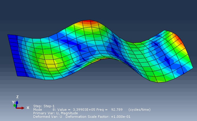
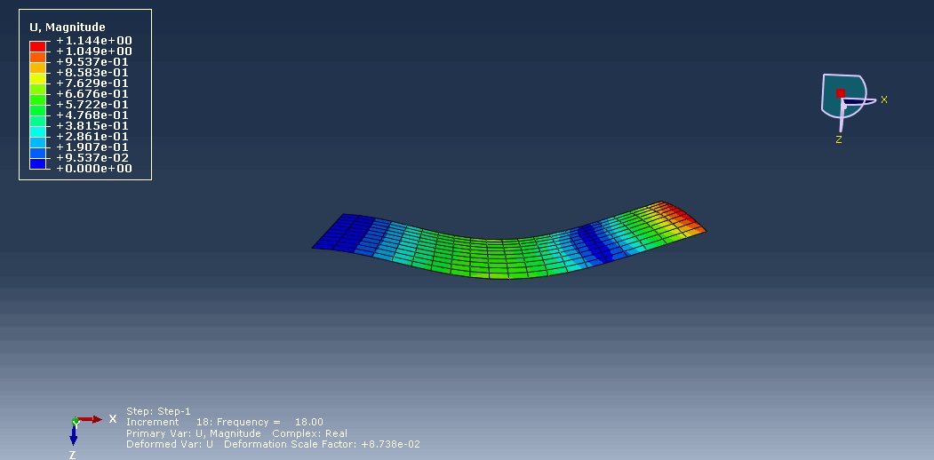
Mode Shapes Visualization:

• Mode 1: Symmetric bending with maximum displacement at the center.
• Mode 2: Antisymmetric bending with nodal lines along the center.
• Mode 3: Diagonal twisting with nodes dividing the sheet.

6. Damping and Real-World Behavior

• Damping reduces vibration amplitude but has minimal effect on natural frequencies.
• In real systems, damping shifts frequencies slightly and introduces complex eigenvalues.

7. Experimental vs. Computational Analysis

• Experimental Modal Analysis: Uses accelerometers and impact hammers to measure frequencies and mode shapes.
• Computational Methods (FEA): Tools like Abaqus solve eigenvalue problems numerically to predict natural frequencies and mode shapes.

natural frequency analysis in Abaqus software

Here’s a step-by-step guide to performing a natural frequency analysis (modal analysis) of an aluminum sheet in Abaqus, including calculating the first 10 natural frequencies and mode shapes:

1. Problem Setup

• Geometry: Rectangular sheet with dimensions 1 m × 0.5 m × 0.003 m.
• Material: Aluminum (Young’s modulus = 70 GPa, Poisson’s ratio = 0.33, Density = 2700 kg/m³).
• Objective: Calculate the first 10 natural frequencies and mode shapes.

2. Step-by-Step Procedure

Step 1: Launch Abaqus/CAE

1. Open Abaqus/CAE.
2. Create a new model database.

Step 2: Create the Geometry

1. Create a Part:
   • Go to Part Module.
   • Click Create Part.
   • Name: Sheet, Type: 3D Deformable, Base Feature: Shell.
   • Approximate size: 1.2 (to accommodate the sheet dimensions).
   • Draw a rectangle with Length = 1 m and Width = 0.5 m.
   • Assign Thickness = 0.003 m.

Step 3: Define Material Properties

1. Create Material:
   • Go to Property Module.
   • Click Create Material, name: Aluminum.
   • Under Mechanical > Elastic, enter:
     • Young’s Modulus: 70e9 Pa (70 GPa).
     • Poisson’s Ratio: 0.33.
   • Under General > Density, enter: 2700 kg/m³.
2. Create Section:
   • Click Create Section, name: Sheet_Section.
   • Category: Shell, Type: Homogeneous.
   • Assign material: Aluminum, Thickness: 0.003.
3. Assign Section to Part:
   • Select the sheet geometry.
   • Click Assign Section and choose Sheet_Section.

Step 4: Mesh the Model

1. Seed the Part:
   • Go to Mesh Module.
   • Click Seed Part, approximate global size: 0.05 m (adjust based on convergence needs).
2. Assign Element Type:
   • Click Assign Element Type.
   • Family: Shell, Element Type: S4R (4-node reduced-integration shell element).
3. Generate Mesh:
   • Click Mesh Part to generate the mesh.

Step 5: Define Boundary Conditions in Abaqus

• Assumption: The sheet is free-free (no constraints).
  (If clamped or supported, apply displacement constraints to edges/faces.)

Step 6: Create a Frequency Step

1. Create Step:
   • Go to Step Module.
   • Click Create Step, name: Frequency_Step, Procedure: Linear perturbation > Frequency.
   • Number of eigenvalues: 10 (to extract first 10 natural frequencies).
   • Keep other settings as default.

Step 7: Submit the Job in Abaqus

1. Create Job:
   • Go to Job Module.
   • Click Create Job, name: Sheet_Frequency.
   • Submit the job.
2. Run the Analysis:
   • Click Submit and monitor the job status.
   • Check the .dat file for errors.

Step 8: Post-Processing

1. Open Results:
   • Go to Visualization Module.
   • Open the output database (Sheet_Frequency.odb).
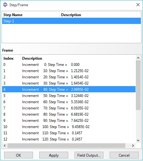
2. Plot Mode Shapes:
   • Click Plot > Deformed Shape.
   • Use the Step/Frame dialog to cycle through the first 10 mode shapes.
3. Extract Frequencies:
   • Go to Report > Field Output.
   • Select Unique Nodal for output variable, choose Eigenfrequency.
   • Save the report to a text file to view the natural frequencies.

3. Key Notes

1. Mesh Sensitivity:
   • Refine the mesh if higher-mode accuracy is critical.
   • Use S4R or S8R elements for shells.
2. Boundary Conditions:
   • For a clamped sheet, fix displacements/rotations on edges.
   • Free-free analysis includes rigid body modes (zero frequency), so extract more eigenvalues.
3. Material Properties:
   • Ensure correct units (Pa for modulus, kg/m³ for density).

4. Python Script for Automation

from abaqus import *
from abaqusConstants import *
from caeModules import *

# Create model and part
mdb.Model(name='Sheet_Frequency')
myModel = mdb.models['Sheet_Frequency']
myPart = myModel.Part(name='Sheet', dimensionality=THREE_D, type=DEFORMABLE_SHELL)
mySketch = myModel.ConstrainedSketch(name='Sketch', sheetSize=1.2)
mySketch.rectangle(point1=(0,0), point2=(1,0.5))
myPart.BaseShell(sketch=mySketch)

# Assign material and section
myMaterial = myModel.Material(name='Aluminum')
myMaterial.Elastic(table=((70e9, 0.33), )
myMaterial.Density(table=((2700, ), ))
mySection = myModel.HomogeneousShellSection(name='Sheet_Section', preIntegrate=OFF,
material='Aluminum', thickness=0.003)
myPart.SectionAssignment(region=myPart.Set(faces=myPart.faces), sectionName='Sheet_Section')

# Mesh
myPart.seedPart(size=0.05)
myPart.setElementType(elemTypes=(ElemType(elemCode=S4R, elemLibrary=STANDARD), ))
myPart.generateMesh()

# Frequency step
myModel.FrequencyStep(name='Frequency_Step', numEigen=10)

# Job submission
myJob = mdb.Job(name='Sheet_Frequency', model='Sheet_Frequency')
myJob.submit()
myJob.waitForCompletion()

results