Birth and Death Welding Simulation in Abaqus Using the DFLUX Fortran Subroutine

Welding is a complex thermal-mechanical process that induces residual stresses and distortions in materials. One of the commonly used techniques to simulate the welding process in Abaqus is the Birth and Death method, which mimics material deposition by sequentially activating finite elements. This method is often coupled with a Fortran DFLUX subroutine to define a moving heat source based on Goldak’s double-ellipsoidal model.

This article provides a detailed guide on implementing the Birth and Death method for a single-pass welding simulation in Abaqus, using Goldak’s heat source model in the DFLUX subroutine.

Welding Theoretical Background

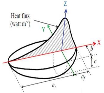
Goldak’s Double-Ellipsoidal Heat Source Model

Goldak’s model is widely used to represent the heat flux distribution in welding simulations. It divides the heat source into two regions:

1. Front Ellipsoid (high penetration region)
2. Rear Ellipsoid (wider heat distribution)

The volumetric heat flux in each region is given by:

Front Heat Source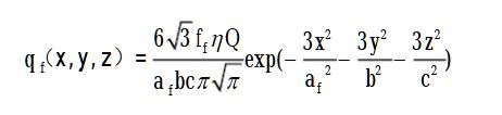 

Rear Heat Source

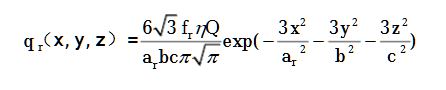
Where:

•  total power input (W)
•  front and rear heat distribution factors
•  shape parameters of the ellipsoids
• coordinates of the heat source
• reference position of the heat source

Birth and Death Method

This method simulates the deposition of weld material by activating elements at different time steps.

1. Initially, weld elements are deactivated (low thermal conductivity or removed).
2. Elements are progressively activated as the heat source moves.
3. A Fortran DFLUX subroutine is used to define the time-dependent heat input.

Welding Implementation in Abaqus

Step 1: Model Setup in Abaqus

1. Create a flat plate geometry in Abaqus.
2. Define material properties (thermal conductivity, density, specific heat, elasticity, plasticity).
3. Partition the weld path into separate element sets (e.g., Weld_Pass1).
4. Mesh the model using fine elements in the weld region (C3D8T elements recommended).

Step 2: Defining Birth and Death Elements

• Deactivate the weld region initially using *MODEL CHANGE, REMOVE.
• Activate elements at different steps using *MODEL CHANGE, ADD.

Example:

** Deactivate weld elements initially
*MODEL CHANGE, REMOVE
Weld_Pass1

** Activate weld elements in Step 1
*MODEL CHANGE, ADD
Weld_Pass1

Step 3: Fortran DFLUX Subroutine

The DFLUX subroutine implements Goldak’s heat source equations.

      SUBROUTINE DFLUX(FILM,COORDS,JTEMP,TEMP,TIME,DTIME,NOEL,NPT,
     1 LAYER,KSPT)
      INCLUDE 'ABA_PARAM.INC'
      DOUBLE PRECISION FILM, COORDS(3), TEMP, TIME(2), DTIME
      INTEGER NOEL, NPT, LAYER, KSPT, JTEMP

      ! Heat source parameters
      DOUBLE PRECISION Q, ff, fr, a, b, cf, cr, x0, y0, z0, x, y, z
      PARAMETER (Q=3000.0, ff=0.6, fr=0.4, a=6.0, b=4.0, cf=3.0, cr=5.0)

      ! Heat source center
      x0 = 5.0 * TIME(1)   ! Moving along x-axis
      y0 = 0.0
      z0 = 0.0

      ! Extract coordinates
      x = COORDS(1) - x0
      y = COORDS(2) - y0
      z = COORDS(3) - z0

      ! Compute front and rear heat flux
      FILM = (6.0 * SQRT(3.0) * ff * Q / (a * b * cf * PI * SQRT(PI))) *
     1 EXP(-3.0 * (x**2 / a**2) - 3.0 * (y**2 / b**2) - 3.0 * (z**2 / cf**2))

      FILM = FILM + (6.0 * SQRT(3.0) * fr * Q / (a * b * cr * PI * SQRT(PI))) *
     1 EXP(-3.0 * (x**2 / a**2) - 3.0 * (y**2 / b**2) - 3.0 * ((z - z0)**2 / cr**2))

      RETURN
      END

Step 4: Load and Step Definitions

1. Define a heat transfer step (*HEAT TRANSFER)
2. Apply the heat flux using DFLUX
3. Include cooling and mechanical analysis steps

Example:

*HEAT TRANSFER, STEADY STATE
1.0, 100.0

Step 5: Running the Welding Simulation

1. Save the Abaqus model.
2. Compile the Fortran subroutine (abaqus job=weld user=dflux.for).
3. Run the simulation and analyze the results.

Step 6: Post-Processing

• Visualize the temperature distribution.
• Plot the thermal cycles at different locations.
• Examine residual stresses and distortions.

Conclusion

The Birth and Death welding simulation in Abaqus effectively models the deposition process by activating elements sequentially. The DFLUX subroutine with Goldak’s heat source model accurately captures the heat input and distribution. This approach helps in predicting residual stresses, distortions, and temperature fields, making it a valuable tool in welding simulations.