Laser–Arc Hybrid Welding Simulation in Abaqus

Hybrid laser welding process compared to laser welding or arc welding can be offer several benefits like deep weld, high welding speed, narrow Heat Affected Zone (HAZ) and increased productivity.

Nowadays, the Finite Element Method (FEM) is a suitable method for the simulation of the welding process phenomena.

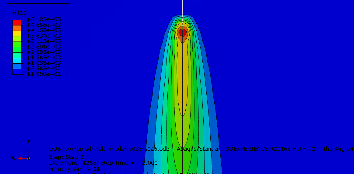
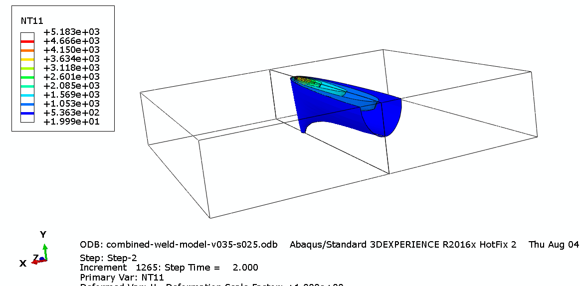
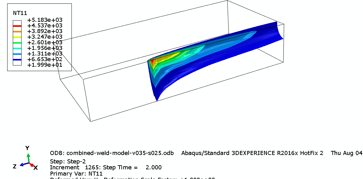
FEM simulation can calculate the weld pool shape, thermal distortion, residual stress, and metallurgical change for various combinations of welding parameters.

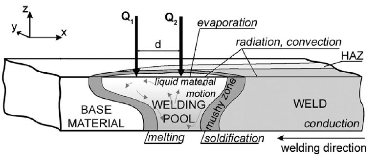
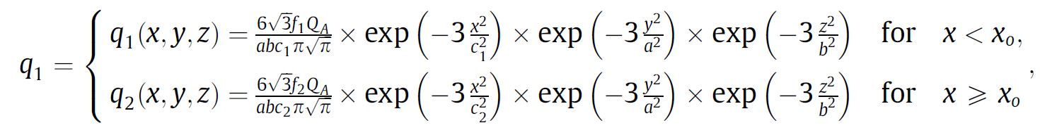
Heat transfer is mostly affected by the amount and distribution of heat input delivered by the laser beam or laser beam and electric arc in hybrid welding. Defined by Goldak  ‘double ellipsoidal’ power distribution of the heat source bellow the welding arc is often used in modeling of arc welding process.

To simulate Laser-Arc Hybrid Welding in Abaqus using the Dflux subroutine, follow these steps:

Hybrid Welding Model Setup in Abaqus

• Geometry: Create a 3D model of the workpiece.
• Mesh: Refine the mesh near the weld zone to capture steep thermal gradients.
• Material Properties:
  • Define thermal properties (conductivity, specific heat, density).
  • Include latent heat for phase change (melting/solidification).
  • Assign these properties to the workpiece.

Thermal Analysis Configuration in Abaqus

• Step: Create a transient heat transfer step with appropriate time increments.
  • Time increment should be small enough to resolve heat source movement (e.g., Δt ≤ element size / welding speed).
• Boundary Conditions:
  • Apply convection and radiation on surfaces using *SFILM and *SRADIATION.
  • Set initial temperature (e.g., 25°C).

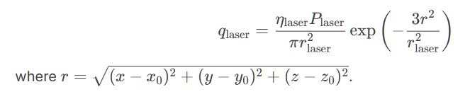
Hybrid laser welding Heat Source Modeling via Dflux Subroutine

The Dflux subroutine combines two heat sources:

1. Laser (Gaussian distribution):
2. Arc (Goldak’s double ellipsoid):
   

Subroutine Workflow:

• Read parameters (power, efficiency, welding speed, etc.) from PROPS.
• Calculate current positions of laser and arc based on welding speed and time.
• For each integration point:
  • Compute distance to both heat sources.
  • Apply Gaussian (laser) and ellipsoidal (arc) heat flux models.
  • Sum contributions: FLUX(1) = q_laser + q_arc.

SUBROUTINE DFLUX(FLUX,TEMP,KSTEP,KINC,TIME,NOEL,NPT,COORDS,JLTYP,
1 TEMP,PRESS,SNAME)
INCLUDE 'ABA_PARAM.INC'
DIMENSION FLUX(2), COORDS(3), TIME(2)
CHARACTER*80 SNAME

! Read parameters from PROPS
eta_laser = PROPS(1)
P_laser = PROPS(2)
r_laser = PROPS(3)
eta_arc = PROPS(4)
a1 = PROPS(5) ! Front ellipsoid
a2 = PROPS(6) ! Rear ellipsoid
b = PROPS(7)
c1 = PROPS(8)
c2 = PROPS(9)
v_weld = PROPS(10)
d_offset = PROPS(11) ! Laser-arc distance

! Current heat source positions
t = TIME(1)
x0_arc = v_weld * t
x0_laser = x0_arc + d_offset

! Integration point coordinates
x = COORDS(1)
y = COORDS(2)
z = COORDS(3)

! Laser heat flux (Gaussian)
dx_laser = x - x0_laser
r_sq = dx_laser**2 + y**2 + z**2
q_laser = (eta_laser*P_laser)/(PI*r_laser**2) * exp(-3*r_sq/r_laser**2)

! Arc heat flux (Goldak)
dx_arc = x - x0_arc
IF (dx_arc >= 0) THEN
a = a1
c = c1
ELSE
a = a2
c = c2
END IF
q_arc = (6*sqrt(3.)*eta_arc*P_arc)/(a*b*c*sqrt(PI**3)) *
exp(-3*(dx_arc**2/a**2 + y**2/b**2 + z**2/c**2))

! Total flux
FLUX(1) = q_laser + q_arc

RETURN
END 

Welding of flat plate in Abaqus
Welding Simulation in Abaqus Using the DEFLUX Fortran Subroutine