Basics of Solving Boundary Layer Flow in CFD

Introduction

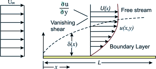
Boundary layer flow is an essential concept in fluid dynamics, especially in aerodynamics, hydrodynamics, and engineering applications. When a fluid flows over a surface, such as an aircraft wing or a pipe wall, the fluid particles close to the surface experience friction and form a thin layer called the “boundary layer.” Understanding boundary layer flow is crucial for predicting drag, heat transfer, and overall fluid behavior.

Computational Fluid Dynamics (CFD) helps engineers and researchers analyze boundary layer flow by solving the fundamental equations of fluid motion. In this article, we will discuss the basics of boundary layer flow, how it is modeled in CFD, and the steps to solve it effectively.

What is Boundary Layer Flow?

When a fluid flows over a solid surface, its velocity varies from zero at the surface (due to the no-slip condition) to the free-stream velocity away from the surface. This region where the velocity gradually increases is known as the boundary layer.

Boundary layer flow is classified into two main types:

• Laminar Boundary Layer: Smooth and orderly flow where fluid particles move in parallel layers.
• Turbulent Boundary Layer: Chaotic and irregular flow with eddies and vortices.

The transition from laminar to turbulent flow depends on the Reynolds number (Re), which is defined as:

Re=ρULμRe = \frac{\rho U L}{\mu} where:

• ρ\rho = Fluid density
• UU = Free-stream velocity
• LL = Characteristic length (such as surface length)
• μ\mu = Dynamic viscosity

A higher Reynolds number generally leads to turbulence.

Governing Equations for Boundary Layer Flow

In CFD, boundary layer flow is modeled using fundamental fluid flow equations:

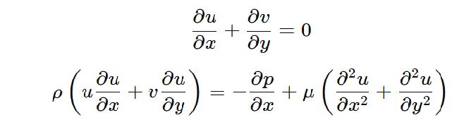
1. Navier-Stokes Equations

These are the basic equations that describe fluid motion, including:

• Conservation of mass (Continuity equation)
• Conservation of momentum (Newton’s Second Law)
• Conservation of energy (First Law of Thermodynamics)

For incompressible flow, the continuity and momentum equations are:

Boundary Layer Approximation

For thin boundary layers, the full Navier-Stokes equations can be simplified using the boundary layer approximations, reducing computational complexity. These equations assume that changes in velocity normal to the surface are more significant than changes along the surface.

Steps to Solve Boundary Layer Flow in CFD

To simulate boundary layer flow in CFD, follow these essential steps:

1. Define the Problem and Geometry

• Choose the object over which the fluid flows (e.g., an airfoil, flat plate, or pipe).
• Create a computational domain around the object.

2. Mesh Generation

• Use a fine mesh near the wall to capture boundary layer effects accurately.
• Implement structured meshing with boundary layer refinement.
• Ensure the y+ value (dimensionless wall distance) is appropriate for the turbulence model:
  • y+ < 1 for wall-resolved turbulence models.
  • 30 < y+ < 300 for wall-modeled turbulence.

3. Select the Turbulence Model

If the flow is turbulent, choosing the right turbulence model is crucial:

• k-ε Model: Suitable for general industrial applications.
• k-ω SST Model: More accurate for boundary layer separation and aerodynamics.
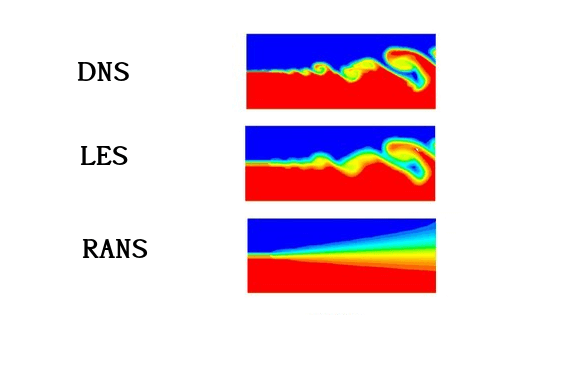
• LES/DNS (Large Eddy Simulation/Direct Numerical Simulation): Used for high-accuracy studies but computationally expensive.

4. Apply Boundary Conditions

• Inlet: Define velocity, pressure, or mass flow rate.
• Outlet: Set pressure outlet or outflow conditions.
• Wall: Apply the no-slip condition and specify wall temperature (if heat transfer is considered).

5. Solve the Equations

• Choose an appropriate solver (steady-state or transient).
• Use under-relaxation factors to ensure numerical stability.
• Iterate until the solution converges (residuals reduce to acceptable levels).

6. Post-Processing and Analysis

• Visualize velocity profiles and boundary layer thickness.
• Calculate skin friction coefficient CfC_f and drag force.
• Compare results with theoretical and experimental data.

Common Challenges and Solutions

1. Capturing Thin Boundary Layers:
   • Use finer meshes near the wall with inflation layers.
   • Use high-resolution turbulence models.
2. Convergence Issues:
   • Reduce the time step or increase mesh refinement.
   • Use better initial conditions or adaptive meshing.
3. High Computational Cost:
   • Use wall functions to reduce computational demand.
   • Employ grid adaptivity to refine only necessary regions.

Additional Explanations

1. Difference Between Heat Boundary Layer and Flow Boundary Layer

• The flow boundary layer refers to the region where the velocity of a fluid changes due to viscosity effects.
• The heat boundary layer refers to the region where temperature gradients exist due to heat transfer between the fluid and the surface.
• In many cases, the heat boundary layer is thinner than the flow boundary layer because thermal diffusivity is different from momentum diffusivity.

2. How to Write a User-Defined Boundary Layer in ANSYS Fluent?

• ANSYS Fluent allows User-Defined Functions (UDFs) to define custom boundary conditions.
• A UDF is written in C programming language and compiled in Fluent.
• Steps to define a UDF boundary layer:
  1. Open Fluent’s UDF editor.
  2. Write a function defining the velocity or temperature profile.
  3. Compile and load the UDF.
  4. Apply the UDF as a boundary condition in Fluent.

Example UDF snippet:

#include "udf.h"

DEFINE_PROFILE(custom_velocity, thread, position)

{

real x[ND_ND];

real y;

face_t f;

begin_f_loop(f, thread)

{

F_CENTROID(x, f, thread);

y = x[1];

F_PROFILE(f, thread, position) = 1.5 * y; // Example velocity profile

}

end_f_loop(f, thread)

}
————————–

3. Options Available in ANSYS Fluent for Boundary Layer in Laminar and Turbulent Flow

• Laminar Flow:
  • Directly solve the Navier-Stokes equations without a turbulence model.
  • Use fine meshing near walls to capture velocity gradients accurately.
• Turbulent Flow:
  • Use turbulence models such as k-ε, k-ω, or Reynolds Stress Model (RSM).
  • Use wall functions for high y+ values or low-Re models for near-wall resolution.
  • Enable Enhanced Wall Treatment for better accuracy.

Conclusion

Solving boundary layer flow in CFD requires an understanding of fluid dynamics, proper meshing techniques, appropriate turbulence modeling, and careful selection of solver settings. By following the steps outlined above and utilizing Fluent’s capabilities, students and engineers can effectively analyze boundary layer behavior and optimize designs for aerodynamics, heat transfer, and industrial applications.

This article provides a fundamental understanding of boundary layer flow in CFD. If you’re a student or beginner, practice with simple simulations (like flow over a flat plate) before moving on to complex cases. Happy simulating!